The QUERY function doesn’t have a direct option to identify the current work week in a date column in Google Sheets. To sum the current work week range using QUERY, we’ll use a workaround approach. First, we’ll mark the dates that fall in the current week, then use that data within the QUERY function. The QUERY function has the DAYOFWEEK scalar function, which will help you filter the current work week from the marked rows.

Learning this approach is quite useful since QUERY is one of the best data manipulation functions in Google Sheets.

Step 1: Marking the Dates that Fall in the Current Week

Assume you have sample data in A1:D, with columns for dates, item, number of trips, and location, which is ideally a material delivery report.

In this dataset, enter the following formula in cell E1 to mark the dates that fall in the current week, from Sunday to Saturday:

=VSTACK("Current Week", ISBETWEEN(A2:A, TODAY()-WEEKDAY(TODAY())+1, TODAY()-WEEKDAY(TODAY())+7))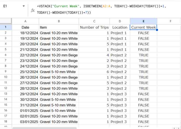

Formula Explanation:

The ISBETWEEN function evaluates the dates in A2:A and returns TRUE if the date falls between TODAY()-WEEKDAY(TODAY())+1 (the start of the week, i.e., Sunday) and TODAY()-WEEKDAY(TODAY())+7 (the end of the week, i.e., Saturday), both inclusive.

Where:

• TODAY()-WEEKDAY(TODAY())+1 returns the week’s start date (Sunday).
• TODAY()-WEEKDAY(TODAY())+7 returns the week’s end date (Saturday).

Step 2: QUERY Formula to Sum Current Work Week Range

Next, you can use the following QUERY formula to total the number of trips that fall in the current work week:

=QUERY(A1:E, "SELECT SUM(Col3) WHERE Col5=TRUE AND DAYOFWEEK(Col1)>=2 and DAYOFWEEK(Col1)<=6 LABEL SUM(Col3)''")

This QUERY formula considers Monday to Friday as the current work week range. If you want Monday to Saturday, replace <=6 with <=7. For a Sunday to Thursday work week, replace >=2 with >=1 and <=6 with <=5.

This is how you can sum the current work week range with QUERY in Google Sheets. Let’s now see how to add additional conditions.

Step 3: Adding Additional Criteria to Sum Current Work Week Range with QUERY

QUERY is one of the best data manipulation functions in Google Sheets, and you can easily specify conditions within it.

For example, to total a specific item (e.g., “Gravel 10-20 mm Beige”) received during the current work week, use the following QUERY formula:

=QUERY(A1:E, "SELECT SUM(Col3) WHERE Col5=TRUE AND DAYOFWEEK(Col1)>=2 and DAYOFWEEK(Col1)<=6 AND Col2='Gravel 10-20 mm Beige' LABEL SUM(Col3)''")

Note: QUERY is case-sensitive. If you want to make it case-insensitive, wrap Col2 with the LOWER function and specify the criterion in lowercase. The formula will then become:

=QUERY(A1:E, "SELECT SUM(Col3) WHERE Col5=TRUE AND DAYOFWEEK(Col1)>=2 and DAYOFWEEK(Col1)<=6 AND LOWER(Col2)='gravel 10-20 mm beige' LABEL SUM(Col3)''")

All the above formulas use the helper column E. Therefore, the actual range A1:D becomes A1:E in the formulas. If you don’t want to use a helper column, replace A1:E with the following formula:

{A1:D, VSTACK("Current Week", ISBETWEEN(A2:A, TODAY()-WEEKDAY(TODAY())+1, TODAY()-WEEKDAY(TODAY())+7))}

Conclusion

You can use SUMIF, SUMIFS, or even SUMPRODUCT to sum a data range based on the current work week in Google Sheets. You can find the SUMIF formula in the resource section below.

What makes QUERY different is its advanced capabilities. When specifying criteria, you can use complex string comparison operators such as CONTAINS, MATCH, STARTS WITH, ENDS WITH, and LIKE for partial matches. You can find these options when you click QUERY in my Google Sheets function guide.

Resources

• How to Sum Values by the Current Week in Google Sheets
• SUMIF to Sum By Current Work Week in Google Sheets
• Filter or Find Current Week This Year and Last Year in Google Sheets
• How to Filter Current Week Horizontally in Google Sheets