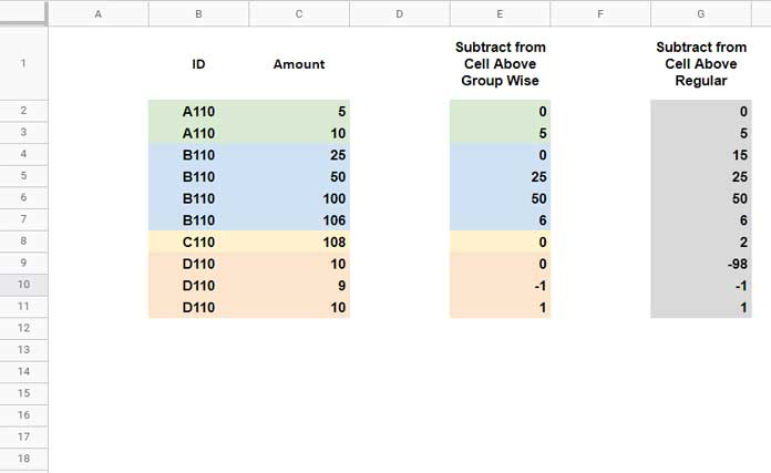
When working with Google Sheets, you may encounter situations where you need to subtract the previous row’s value from the current row’s value. This is useful for analyzing changes in data, such as tracking differences over time.

In this tutorial, you’ll learn how to perform this calculation using the MAP lambda helper function (LHF), which allows us to work with multiple arrays efficiently. While other LHFs like SCAN or BYROW can also be used, MAP provides additional flexibility when dealing with grouped data.

Subtracting the Previous Row’s Value

Example: Simple Row-Wise Subtraction

Assume you have numerical data in column C and want to subtract each value from the one above it. Here’s how to do it using an array formula:

Formula using MAP:

={0; MAP(C3:C11, LAMBDA(r, r - OFFSET(r, -1, 0)))}

This formula subtracts the previous row’s value from the current row’s value. You can also achieve the same result using BYROW:

Formula using BYROW:

={0; BYROW(C3:C11, LAMBDA(r, r - OFFSET(r, -1, 0)))}

Or using SCAN:

Formula using SCAN:

={0; SCAN(, C3:C11, LAMBDA(a, r, r - OFFSET(r, -1, 0)))}

How These Formulas Work:

• r represents the current row’s value.
• OFFSET(r, -1, 0) retrieves the previous row’s value.
• The formulas iterate over the range, computing the difference for each row.

When using these formulas, if the range is C2:C11, you should specify C3:C11, one row less.

Handling Dynamic Ranges

If your dataset extends dynamically, replace C3:C11 with an open-ended range:

={0; MAP(C3:INDEX(C3:C, MATCH(2, 1/(C3:C<>""), 1)), LAMBDA(r, r - OFFSET(r, -1, 0)))}

This ensures the formula adjusts to the last non-blank row.

Subtracting the Previous Row’s Value by Group

When working with grouped data, such as multiple categories in column B (e.g., IDs), we need to reset the subtraction at each group boundary. The following formula achieves this:

={0; MAP(B3:B11, C3:C11, LAMBDA(_, r, IF(COUNTIF(B2:_, _) = 1, 0, r - OFFSET(r, -1, 0))))}

How It Works:

• COUNTIF(B2:_, _) checks if the current row is the first occurrence of its group.
• If it’s the first occurrence, return 0; otherwise, subtract as usual.

Key Takeaways

• MAP, BYROW, and SCAN can all perform row-wise subtraction, but MAP allows working with multiple arrays.
• Dynamic ranges can be handled using INDEX and MATCH.
• Grouped calculations require an additional condition to reset subtraction at group boundaries.

This method is efficient and avoids the need for helper columns or manual calculations. Try it out in your Google Sheets workflows!