")
")


")


")

")
")
 in Excel & Google Sheets")


Want to subtract one duration from another in Google Sheets, whether the durations are in cells or hardcoded into a formula? It’s easier than you think, but there are a few key details to know, especially when dealing with formatting or avoiding negative time values.
This guide shows you multiple ways to subtract durations, format the result, and handle edge cases like negative values. Let’s break it down.
Subtract Duration When Both Values Are in Cells
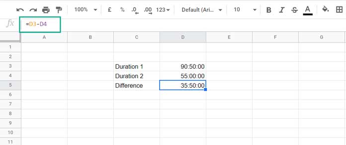
If you have two durations in cells, for example, D3 and D4, you can simply use a subtraction formula:
=D3-D4Google Sheets will automatically handle the calculation as long as both cells are formatted as durations.
Subtract Duration When One Value Is Hardcoded
Let’s say the first duration is in cell D3, and the second one is hardcoded (e.g., 55 hours):
=D3 - VALUE("55:00:00")Why Use VALUE?
The VALUE function converts the text "55:00:00" into a numeric duration that Google Sheets can subtract. Avoid using TIMEVALUE, which only works with time formats like hh:mm:ss and won’t handle longer durations like 55:00:00 correctly.
Subtract Duration When Both Values Are Hardcoded
If both durations are fixed, you can use:
=VALUE("90:50:00") - VALUE("55:00:00")Important: Google Sheets will return a decimal number (like 1.49305) because it sees the result as a fraction of a day.
Format as Duration
To format the result as a duration:
- Go to Format > Number > Duration
This will convert 1.49305 into the correct time format, like 35:50:00.
If you don’t want to apply the formatting manually, you might consider using the TEXT function. While that works, it returns a text value—not an actual duration.
A better alternative is to use the QUERY function with a formatting clause:
=QUERY(VALUE("90:50:00") - VALUE("55:00:00"), "format Col1 '[h]:mm:ss'")This keeps the result as a proper duration while applying the desired display format.
Return 0 If the Result Is Negative
If subtracting one duration from another gives a negative result (e.g., "55:00:00" - "90:50:00"), you may want to return 0 instead of a negative duration.
Use this formula:
=MAX(0, VALUE("55:00:00") - VALUE("90:50:00"))How It Works
The MAX function returns the larger of the two values. If the subtraction result is negative, MAX will return 0.
Final Thoughts
Whether you’re tracking work hours, time differences, or durations between tasks, this guide helps you subtract durations from each other in Google Sheets accurately. Use VALUE to hardcode time, format your results correctly, and use MAX to avoid negative outputs.