There isn’t a specific function in Google Sheets specifically for analyzing transactions proportionally within specified date ranges (start and end dates). However, this capability is frequently needed.
In this tutorial, I’ve covered two different examples:
- Expenses incurred for specific durations: The goal is to return the total expenses for any period (time frame) by providing a start and end date.
- Rentals received monthly but contracted for specific durations: The objective here is to find the total payments generated from these rentals for a specific duration, considering the agreement period.
The formula is scalable, so you do not need to worry about how you record expenses or income, whether weekly, fortnightly, bi-monthly, yearly, etc.
If you record your transactions daily, you can use the SUMIFS function directly to analyze transactions by date range in Google Sheets.
For example, you can use the following SUMIFS formula to total the expenses from January 1, 2024, to June 30, 2024:
=SUMIFS(B:B, A:A, ">="&DATE(2024, 1, 1), A:A, "<="&DATE(2024, 6, 30))Where expenses are in column B and the dates of expenses are in column A.
When analyzing transactions with start and end dates that don’t perfectly align with your desired time frame, you can calculate the total proportionally based on the days that fall within both periods.
We’ll explore two examples below to demonstrate this technique.
Example 1: Analyze Expenses by Date Range in Google Sheets
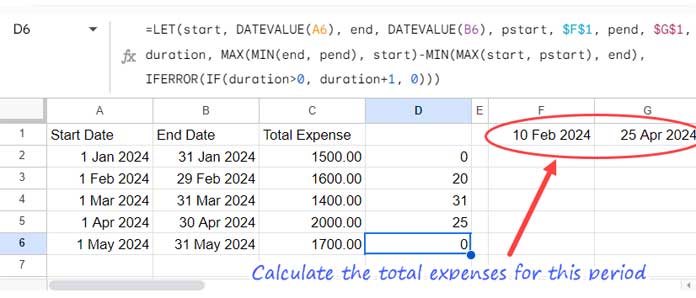
In the following example, we have start dates in column A and end dates in column B. The corresponding expenses are in column C.
| Start Date | End Date | Total Expense |
| 1 Jan 2024 | 31 Jan 2024 | 1500.00 |
| 1 Feb 2024 | 29 Feb 2024 | 1600.00 |
| 1 Mar 2024 | 31 Mar 2024 | 1400.00 |
| 1 Apr 2024 | 30 Apr 2024 | 2000.00 |
| 1 May 2024 | 31 May 2024 | 1700.00 |
Assume you want to calculate the total expenses incurred from 10 Feb 2024 (in cell F1) to 25 Apr 2024 (in cell G1). How do you find it?
Here are step-by-step instructions for analyzing transactions by date range (start and end date) in Google Sheets:
Step 1: Calculate the Number of Days that Fall in the Asked Duration
In cell D2, enter the following formula and drag the fill handle down as far as needed:
=LET(start, DATEVALUE(A2), end, DATEVALUE(B2), pstart, $F$1, pend, $G$1, duration, MAX(MIN(end, pend), start)-MIN(MAX(start, pstart), end), IFERROR(IF(duration>0, duration+1, 0)))
When you use this formula, replace A2, B2, $F$1, and $G$1 with the cell addresses corresponding to expense start, expense end, time frame start, and time frame end.
This formula calculates the number of expense days that fall within the specified start and end dates (pstart to pend), inclusive.
Step 2: Calculate the Expenses Proportionate to the Duration
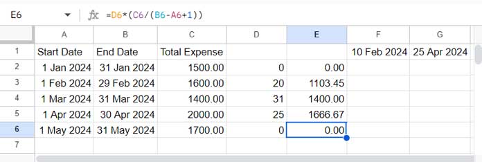
In cell E2, enter the following formula and drag it down as far as needed:
=D2*(C2/(B2-A2+1))
Where (C2/(B2-A2+1)) returns the per-day expense.
When you use this formula, replace A2, B2, C2, and D2 with the cell references of expense start, expense end, expense amount, and proportionate days calculated in step 1.
This formula calculates the expenses proportionally based on the number of days (D2) in the specified time frame.
The total in column E, i.e., =SUM(E2:E), will give you the total expenses for the specified duration.
Step 3: Combining Step 1 and Step 2 Formulas
Instead of using two separate formulas, you can combine them for simplicity. In cell D2, use the following formula and drag it down as far as needed:
=LET(start, DATEVALUE(A2), end, DATEVALUE(B2), pstart, $F$1, pend, $G$1, duration, MAX(MIN(end, pend), start)-MIN(MAX(start, pstart), end), IFERROR(IF(duration>0, duration+1, 0)*(C2/(end-start+1))))This combined formula simplifies the process and calculates the total expenses proportionally for the specified time frame in one step.
This concludes our first example of analyzing transactions by date range (time frame) in Google Sheets.
Example 2: Analyze Income by Date Range in Google Sheets
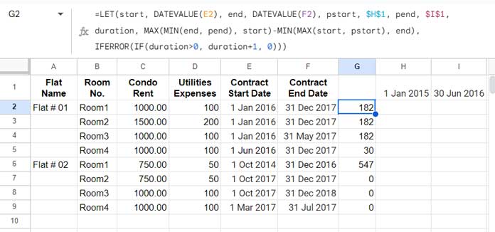
Assume you rent two flats and each has 4 rooms. You collect monthly rentals and utility expenses from each tenant.
Each tenant has signed a contract for specific periods.
How do you calculate the amount receivable for a specific duration (time frame)?
| Flat Name | Room No. | Condo Rent | Utilities Expenses | Contract Start Date | Contract End Date |
| Flat # 01 | Room1 | 1000.00 | 100 | 1 Jan 2023 | 31 Dec 2024 |
| Room2 | 1500.00 | 200 | 1 Jan 2023 | 31 Dec 2024 | |
| Room3 | 1000.00 | 100 | 1 Jan 2023 | 31 May 2024 | |
| Room4 | 1000.00 | 100 | 1 Jun 2023 | 31 Dec 2024 | |
| Flat # 02 | Room1 | 750.00 | 50 | 1 Oct 2021 | 31 Dec 2023 |
| Room2 | 750.00 | 50 | 1 Oct 2024 | 31 Dec 2024 | |
| Room3 | 1000.00 | 100 | 1 Oct 2024 | 31 Dec 2025 | |
| Room4 | 1000.00 | 100 | 1 Mar 2024 | 31 Jul 2024 |
The data is in columns A to F, and the specific duration for which to calculate the receivables will be in H1 (start date) and I1 (end date).
Steps
You can use the step 1 formula from the previous example to calculate the days. You only need to correctly specify the start, end, pstart, and pend cells.
In cell G2, enter the following formula and drag the fill handle down as far as needed:
=LET(start, DATEVALUE(E2), end, DATEVALUE(F2), pstart, $H$1, pend, $I$1, duration, MAX(MIN(end, pend), start)-MIN(MAX(start, pstart), end), IFERROR(IF(duration>0, duration+1, 0)))
This formula calculates the number of days that fall within the specified time frame (pstart to pend), inclusive.
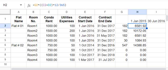
Enter this formula in cell H2 and drag it down as far as needed:
=G2*((C2+D2)*12/365)
This formula calculates the receivables proportionally based on the number of days (G2) in the specified duration relative to the per-day expense. Here, (C2+D2)*12/365 calculates the per-day expense.
The total in column H, i.e., =SUM(H2:H), will give you the total amount receivable during the start and end dates specified in H1:I1.
Similar to example #1, we can combine the step 1 and step 2 formulas here as well.
=LET(start, DATEVALUE(E2), end, DATEVALUE(F2), pstart, $H$1, pend, $I$1, duration, MAX(MIN(end, pend), start)-MIN(MAX(start, pstart), end), IFERROR(IF(duration>0, duration+1, 0)*(C2+D2)*12/365))This combined formula calculates the total receivables for the specified duration in one step.
Note: The formula can handle contracts with start and end dates that fall outside or within the time frame you’re calculating receivables for (e.g., contracts starting before or ending after the specified duration).
Scalable Formula for Analyzing Transactions by Date Range
The example 1 formula is scalable for analyzing transactions by date range. It allows adaptation for various recording methods, whether it’s weekly, fortnightly, bi-monthly, yearly, etc.
It calculates the per-day expense from the expense duration. Therefore, in columns A and B, you need not stick to month start and end dates. It can be any duration.
Resources
- Summarize Data by Week Start and End Dates in Google Sheets
- Creating Month Wise Summary in Google Sheets (Query Formula)
- How to Create a Weekly Summary Report in Google Sheets
- Query to Create Daily/Weekly/Monthly/Quarterly/Yearly Report Summary in Google Sheets
- Rolling Months Backward Summary in Google Sheets


