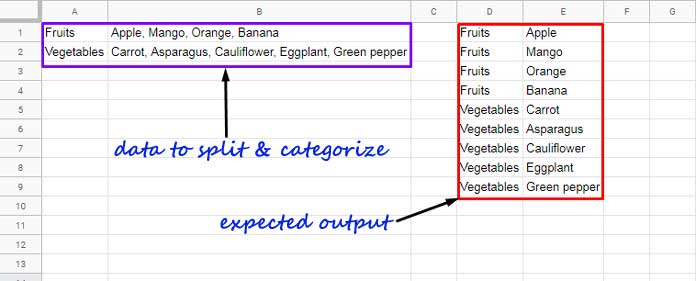
It’s common to come across comma-separated lists that need to be organized and categorized for better readability and analysis. For example, you may have a list of items—like fruits or vegetables—stored as a comma-separated string in one column, with a corresponding category label in another.

To make this data more manageable, you can split values by category in Google Sheets and lay them out into two clean columns: one for the category and one for each individual item.

In this guide, you’ll learn how to split values by category into two columns in Google Sheets, transforming your comma-separated lists into a structured format that’s easier to analyze and filter.

Formula to Split Values by Category into Two Columns in Google Sheets

Here’s a formula that splits text into columns and categorizes the results in Google Sheets:

=LET(
   data, ARRAYFORMULA(SPLIT(FLATTEN(cat&"|"&SPLIT(items, ", ", FALSE)), "|")), 
   SORT(FILTER(data, CHOOSECOLS(data, 2)<>""))
)

Replace items with the range containing the comma-separated values, and cat with the corresponding category label range.

Features of This Formula

• ✅ No LAMBDA required — Resource friendly
• ✅ Array formula — processes the entire dataset at once; no need to drag down
• ✅ Sorted output — categories appear in ascending order
  • If you want to keep the original row order, replace: SORT(FILTER(data, CHOOSECOLS(data, 2) <> "")) with: FILTER(data, CHOOSECOLS(data, 2) <> "")

How to Split and Categorize Comma-Separated Data in Google Sheets

In the example below, column A contains category labels (e.g., Fruits, Vegetables) and column B contains the corresponding comma-separated items.

Split to Column and Categorize Multiple Rows of Values

Paste the following formula in cell D1:

=LET(
   data, ARRAYFORMULA(SPLIT(FLATTEN(A1:A&"|"&SPLIT(B1:B, ", ", FALSE)), "|")), 
   SORT(FILTER(data, CHOOSECOLS(data, 2)<>""))
)

Formula Logic Explained

Here’s how the formula works to split values by category in Google Sheets:

• SPLIT(B1:B, ", ", FALSE) – splits the comma-separated values using ", " as the delimiter.
  If your values are just comma-separated (no space), use "," instead.
• A1:A&"|"& ... – combines each category with each corresponding item using a pipe (|) as a delimiter.
• FLATTEN(...) – flattens the combined results into a single column like this:

Fruits|Apple
Fruits|Mango
Fruits|Orange
Fruits|Banana
Fruits|
Vegetables|Carrot
Vegetables|Asparagus
Vegetables|Cauliflower
Vegetables|Eggplant
Vegetables|Green Pepper

• SPLIT(..., "|") – separates each string into two columns: Category and Item.
• FILTER(data, CHOOSECOLS(data, 2) <> "") – removes any rows where the item column is blank.
• SORT(...) – sorts the final result by category.

And that’s how you split values by category into two columns in Google Sheets—clean, dynamic, and fully formula-based!

Resources

• Split Your Google Sheet Data into Category-Specific Tables
• How to Split a Number into Digits in Google Sheets
• Split a Column into Multiple N Columns in Google Sheets
• Split Numbers from Text Without Delimiters in Google Sheets
• Split a Text after Every Nth Word in Google Sheets (Using Regex and Split)
• Split and Count Words in Google Sheets (Array Formula)
• Split Comma-Separated Values in a Multi-Column Table in Google Sheets
• Split Text in Google Sheets Without Losing Formatting (Preserve Zeros & Hex)
• Dynamic Formula: Split a Table into Multiple Tables in Google Sheets