There is one issue with the SPLIT function that you may face at some point in your Spreadsheet use. That is related to getting the split result in text format in Google Sheets.

As you may already know, we can split a text into columns in two ways in Google Sheets. Using the Data > Split text to columns command or the Split function.

Both will cause some issues with some text strings. I have faced this issue on two occasions.

1. Splitting a text that contains hexadecimal numbers separated by delimiters.

2. Splitting a text that contains item code numbers separated by delimiters. Here the issue is because of the leading zeros in numbers.

In the above two scenarios, why should one want to get the split result in text format?

In the first scenario, after the split, some of the split text got converted to scientific notations because Google Sheets converts hexadecimal (not all) numbers like that. I’ll give detail in the example part below.

In the second scenario, the item codes got converted to numbers, and so the leading zeros were missing.

The above is the one Split function behavior that I want to avoid in Google Sheets. By tweaking the formula a little bit, we can get the Split Result in Text Format in Google Sheets

How to Keep the Split Result in Text Format in Google Sheets

Split Syntax:

SPLIT(text, delimiter, [split_by_each], [remove_empty_text])

Two Split Problems in Google Sheets

Assume you have hexadecimal numbers combined using a pipe delimiter. For the example, we can consider the following numbers in cell B6 – “9C40|3E80|4FB0|DDA|40D8|4E20”.

I am splitting the text as below to separate the hexadecimal numbers.

=split("9C40|3E80|4FB0|DDA|40D8|4E20","|")

The result will be as follows (in the following screenshot, please refer to the range B8:G8).

As you can see, Google Sheets converted the second and sixth hexadecimal numbers to scientific notations. So, if I want, I won’t be able to convert them to decimals as below.

=ArrayFormula(hex2dec(split("9C40|3E80|4FB0|DDA|40D8|4E20","|")))

The above HEX2DEC formula will return the #NUM error against the second and sixth values (please refer to the range B11:G11 below).

Formulas:

1. =textjoin("|",true,ArrayFormula(DEC2HEX(B4:G4)))

2. =split(B6,"|")

3. =ArrayFormula(hex2dec(split("9C40|3E80|4FB0|DDA|40D8|4E20","|")))

Another issue is related to item codes. Here I have four codes combined with a hyphen as follows – “0001200-0001201-0001202-0001203”

=split("0001200-0001201-0001202-0001203","-")

Here the split formula would return the following numbers.

The leading zeros are missing! You can try the function TO_TEXT in combination with Split as below to keep the split result in text format in Google Sheets. But that is not going to help.

=ArrayFormula(to_text(split("0001200-0001201-0001202-0001203","-")))

The output will be text. But it won’t preserve the leading zeros. So let’s go the formula to keep the split result in text format without compromising any characters in Google Sheets.

The Solution to Keep the Split Result in Text Format without Loss of Characters

In the string that you want to split, identify the delimiter (separator). Assume it is the Pipe. Then you should replace it with a Pipe and an apostrophe as below.

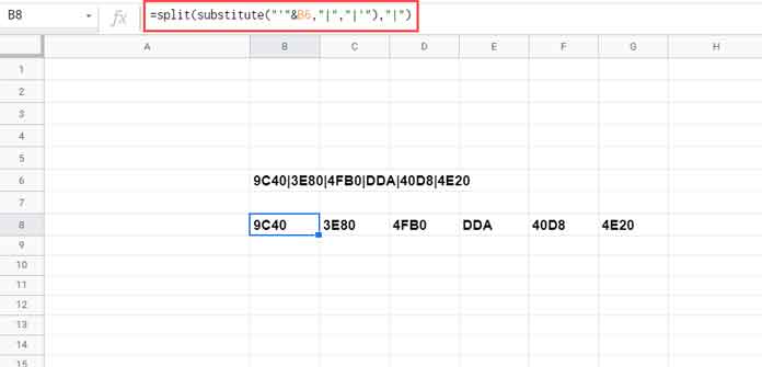
=split(substitute("'"&B6,"|","|'"),"|")

I have used the SUBSTITUTE function to replace the delimiter | with |'. Additionally added an apostrophe at the beginning of the string using "'"&.

This way, you can split a text and keep the result in text format without any loss of characters in Google Sheets.

When you hardcode the string into the formula, it would be as below.

=split(SUBSTITUTE("'9C40|3E80|4FB0|DDA|40D8|4E20","|","|'"),"|")

Regarding our item codes (product IDs), we can use split formula as per the above pattern. Only the delimiter is different here.

=split(SUBSTITUTE("'0001200-0001201-0001202-0001203","-","-'"),"-")

That’s all. Thanks for the stay. Enjoy!