Split Comma-Separated Values in a Multi-Column Table (Google Sheets)

This post explains how to correctly split comma-separated values in a multi-column table in Google Sheets. In this approach, the first column contains comma-separated values, and the other columns hold corresponding data that are not separated by commas.

If you are looking for the Cartesian product from multi-column comma-separated values, you may follow this tutorial instead: Create All Combinations from Comma-Separated Columns in Google Sheets.

Table of Contents

Introduction

Google Sheets offers two built-in options to separate values in a column based on delimiters:

Using the SPLIT function.
Using the Data → Split text to columns menu option.

The first is a formula-based approach, which comes with the benefit of being dynamic and easy to reuse.

For example, you can use the TRANSPOSE function with SPLIT to change the data orientation after the split.

To split comma-separated values in a multi-column table in Google Sheets, we will mainly use the SPLIT function.

Why Split Multi-Column Comma-Separated Values in Google Sheets?

Assume we want to assign the same score to multiple people. One way is to enter their names comma-separated in one cell and their score in another cell.

a) Type #1 – Comma-Separated Names in One Cell

Name	Score
A, B, C	95
D	94

The other way is to list each name in its own row, repeating the score for each person.

b) Type #2 – One Name per Row

Name	Score
A	95
B	95
C	95
D	94

Type #2 has one big advantage — we can easily aggregate it using QUERY, a Pivot Table, or functions like SUMIF and XLOOKUP since it’s already in a database-like structure.

Type #1, however, saves rows and is more compact, which can be useful when printing or scanning data.

If your data entry operator has entered the dataset in Type #1, can we convert it to Type #2?

Yes! Let’s start with the basics of splitting comma-separated values in Google Sheets.

Split Comma-Separated Values in a Single Column in Google Sheets

If you only have one column of comma-separated values (like the first column in Type #1), you can use:

=ArrayFormula(TRANSPOSE(TRIM(SPLIT(TEXTJOIN(",", TRUE, A1:A3), ","))))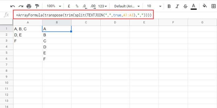

Google Sheets formula to split comma-separated values in a single column

Explanation:

TEXTJOIN – Joins all values in A1:A3 into one string using the existing delimiter (comma).
SPLIT – Splits that string into separate values.
TRIM – Removes any extra spaces after commas.
TRANSPOSE – Converts the single-row result into a single column.

Split Comma-Separated Values in a Multi-Column Table in Google Sheets

Now for the main topic — splitting comma-separated values in a multi-column table in Google Sheets.

Two-Column Table Example

Sample data in A2:B6 (formula will use A2:B1000 to cover more rows):

=QUERY(
  ArrayFormula(
    SPLIT(
      TRIM(FLATTEN(SPLIT(A2:A1000, ",") & "🐠" & B2:B1000)),
      "🐠"
    )
  ),
  "SELECT * WHERE Col2 IS NOT NULL"
)

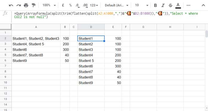
Split comma-separated values in a multi-column table in Google Sheets – two-column result

This formula:

Splits the first column values by comma.
Appends the second column value to each split entry using a delimiter (🐠).
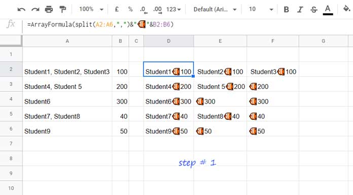
Uses FLATTEN to turn all results into a single column.
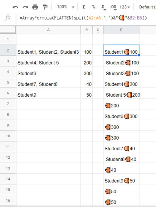
Splits again by 🐠 to separate names from scores.
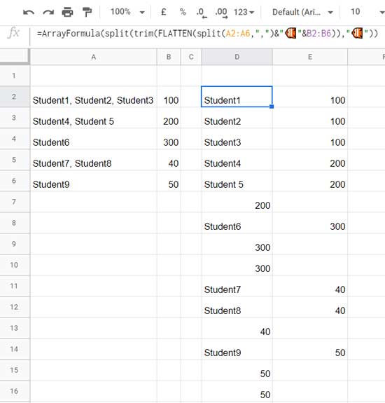
Filters out rows where the second column is blank.

You can replace 🐠 with any delimiter, such as a pipe symbol (|).

Three (or More) Columns

For a three-column table (A2:C1000):

=QUERY(
  ArrayFormula(
    SPLIT(
      TRIM(FLATTEN(SPLIT(A2:A1000, ",") & "🐠" & B2:B1000 & "🐠" & C2:C1000)),
      "🐠"
    )
  ),
  "SELECT * WHERE Col3 IS NOT NULL"
)

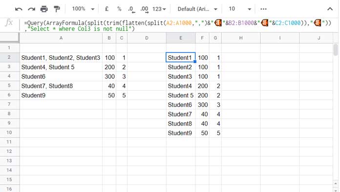
Split comma-separated values in a multi-column table in Google Sheets – three-column example

Changes:

Add &"🐠"&C2:C1000 in Step 2 for the third column.
In the QUERY step, check Col3 IS NOT NULL instead of Col2.

Repeat the pattern for more columns, updating both the concatenation and the column number in the QUERY.

Alternative Formula to Split Comma-Separated Values in a Multi-Column Table (Without FLATTEN)

Before the FLATTEN function was introduced, here’s how you could achieve the same result for a two-column table:

=ArrayFormula(
  SPLIT(
    TRANSPOSE(
      TRIM(
        SPLIT(
          TEXTJOIN("🌼", 1,
            IF(LEN(A2:A1000),
              REGEXREPLACE(A2:A1000 & ",",  ",",  "🌼" & B2:B1000 & ","),
            )
          ),
          ","
        )
      )
    ),
    "🌼"
  )
)

Logic:

REGEXREPLACE inserts 🌼 and the second column’s value before each comma.
After transformation, split twice — first by comma, then by 🌼.

For three columns, extend:

=ArrayFormula(
  SPLIT(
    TRANSPOSE(
      TRIM(
        SPLIT(
          TEXTJOIN("🌼", 1,
            IF(LEN(A2:A1000),
              REGEXREPLACE(A2:A1000 & ",", ",", "🌼" & B2:B1000 & "🌼" & C2:C1000 & ","),
            )
          ),
          ","
        )
      )
    ),
    "🌼"
  )
)

Conclusion

You now know how to split comma-separated values in a multi-column table in Google Sheets using two different approaches — with and without FLATTEN. The formulas scale to multiple columns, making them ideal for transforming compact datasets into database-friendly formats.