If you’re trying to fill sequential dates in Google Sheets but need to skip hidden rows, a regular SEQUENCE formula won’t cut it. By default, Sheets fills every row — visible or not — which can mess up your data if you’ve hidden some rows for notes or structure.

In this post, I’ll show you how to use a formula that fills only the visible rows with sequential dates, leaving hidden rows completely blank. It’s easier than you might think once you use the right tools.

Why You Might Want to Skip Hidden Rows

Let’s say you have a sales report where each row represents one day’s transaction. Pretty standard. But once in a while, you insert extra rows under certain entries to jot down notes — maybe a quick comment about a cash payment, a discount given, or a customer request. These note rows aren’t part of the actual data, so you hide them to keep your sheet clean.

Now, you want to add a column with sequential dates, starting from, say, January 1, 2025 — but only for the visible transaction rows. If you use the fill handle or a simple SEQUENCE, it fills every row, even the hidden ones — which throws off the sequence and clutters up your notes.

What you really need is a way to auto-fill dates in just the visible rows, and skip over anything hidden — whether it’s a filtered row, a manually hidden note, or grouped content.

Sample Data

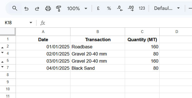
Here’s a simplified example to illustrate the problem:

In this sheet, we’ve hidden the rows with notes so only the real transaction data is visible. We want to generate one date per visible row, like this:

Formula to Fill Sequential Dates While Skipping Hidden Rows

To auto-fill sequential dates skipping hidden rows, enter the following formula in cell A2:

=ARRAYFORMULA(IF(B2:B="",,MAP(B2:B, LAMBDA(Σ, DATE(2025, 1, SUBTOTAL(103, B2:Σ))))))

This formula uses SUBTOTAL(103, ...) to count only visible rows, ensuring that dates are assigned only where appropriate.

Important Notes:

This formula assumes that column B contains your main transaction data — the part you want to track with sequential dates.

If there are blank cells in column B, the formula might skip those rows, even if they’re visible. That’s because it treats blanks as rows to ignore.

To avoid this, you can use a helper column — let’s say column E — that generates a clean sequence for all rows up to the last non-blank row in column B. In cell E2, enter:

=ArrayFormula(SEQUENCE(ROW(XLOOKUP(TRUE, B2:B<>"", B2:B,,0, -1))))

This creates a numeric sequence that stops at the last non-empty row in column B. Once added, you can hide column E to keep your sheet clean.

Then, update your main date formula by replacing B2:B with E2:E, and B2 with E2, like so:

=ARRAYFORMULA(IF(E2:E="",,MAP(E2:E, LAMBDA(Σ, DATE(2025, 1, SUBTOTAL(103, E2:Σ))))))

This version ensures sequential dates are filled only for visible rows, regardless of blanks in column B.

How This Formula Works

Let’s break down the formula:

=ARRAYFORMULA(
   IF(B2:B="",,
      MAP(B2:B, LAMBDA(Σ, 
         DATE(2025, 1, SUBTOTAL(103, B2:Σ)))
      )
   )
)

• ARRAYFORMULA: Enables formula to work on a range.
• IF(B2:B="",,): Skips blank rows.
• MAP(B2:B, LAMBDA(...)): Loops through each visible row in column B.
• SUBTOTAL(103, B2:Σ): Counts only visible rows using function code 103 (COUNTA for visible cells only).
• DATE(2025, 1, ...): Returns the sequential date by adding the visible row count as the day of the month.

Conclusion

Filling sequential dates while skipping hidden rows in Google Sheets is a powerful trick when you’re working with filtered or annotated datasets. Whether you’re managing reports, logs, or schedules, this formula helps keep your data clean and dynamic.

Let me know in the comments if you’ve tried this or have variations to share!

Resources and Related Tutorials

If you’re working with sequential dates in different formats, check out these helpful tutorials:

• Find Missing Sequential Dates in a List in Google Sheets
• How to Populate Sequential Dates Excluding Weekends in Google Sheets
• Auto-Fill Sequential Dates When Cell Is Filled in Google Sheets
• How to Generate Bimonthly Sequential Dates in Google Sheets
• Creating Sequential Dates in Equally Merged Cells in Google Sheets
• Date Sequence Every Nth Row in Excel (Dynamic Array)