Google Sheets Sales Calendar: Top 3 Highlighting (Daily, Weekly, Monthly)

Do you want to highlight the top 3 performing days, weeks, or months in a yearly calendar based on sales quantity or amount with distinct colors? You’re in the right spot! Here, you’ll get a dynamic sales calendar template with a top 3 highlighting option in Google Sheets.

About the Sales Calendar with Top 3 Highlighting Template

The template is simple to use. In one sheet, you enter the transaction dates in one column, item names in another column, and quantity or sales amount in the third column. The dates and quantity/amount columns are required, while the item column is optional, as the focus is on days, weeks, or months.

In the second sheet, the sales calendar, you select the year in one drop-down and the highlighting category (day, week, or month) in another. Your selection will highlight the top three performing individual dates, weeks, or months.

Example of a sales calendar highlighting the top 3 performing days, weeks, or months

How to Use the Sales Calendar with Top 3 Highlighting

Data Sheet in the Template

The sales calendar template with the top 3 highlighting consists of three sheets:

“Sales”: The data sheet where you enter transaction records.
“Sales Calendar”: The sheet displaying the highlighted calendar.
“©”: Contains the fair use policy.

Data Entry in the Sales Sheet:

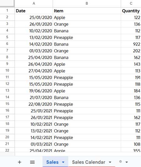
Enter transaction dates in column A.
Enter item names in column B (optional).
Enter quantity or sales amount in column C.

If your focus is revenue generation, highlight the top 3 sales based on total sales value. If tracking product popularity, rank by quantity.

Note: Do not insert or delete columns in this sheet, as it may break the formulas in use.

Sales Calendar Sheet in the Template

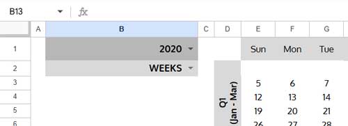
The “Sales Calendar” sheet contains a dynamic yearly calendar where highlighting occurs.

In cell B1, select the year to adjust the calendar.
In cell B2, select “Days,” “Weeks,” or “Months” to determine the top-selling timeframes.
The top 3 performing days, weeks, or months will be highlighted accordingly.

Drop-down menus to select the year and highlighting timeframes in the sales calendar

Color Codes for Highlighting:

Green: Rank 1
Red: Rank 2
Orange: Rank 3

Tie-Breaking in Sales Calendar with Top 3 Highlighting

Since highlighting is applied to a calendar rather than a sales column, our goal is to visualize top-performing days, weeks, or months at a glance.

For example, if Week 1 in January and Week 3 in April both have a top performance score of 1000, they are considered tied. Both will be highlighted in green rather than one in green and the other in red.

This means the ranking is based on unique figures: rank 1, 2, and 3. Any duplicates of these figures will receive the same color.

Formulas Used for Data Manipulation in the Sales Sheet

Formula in Cell J2:

=ArrayFormula(IF(A2:A="",,EOMONTH(A2:A, 0)))

Purpose: Convert sales dates in A2:A to the corresponding end-of-month dates for monthly summarization.

Formula in Cell K2:

=ArrayFormula(IF(A2:A="",,WEEKNUM(A2:A)))

Purpose: Converts sales dates in A2:A to corresponding week numbers for weekly summarization.

Formula in Cell N1:

=SWITCH('Sales Calendar'!B2, "DAYS", 1, "MONTHS", 10, "WEEKS", 11)

Purpose: Returns column numbers based on the selection in ‘Sales Calendar’!B2:

1: Sales dates (Column A)
10: End of the month (Column J)
11: Week number (Column K)

Formula in Cell O1:

=SORTN(QUERY(Sales!A2:K, "Select Col"&N1&",sum(Col3) where year(Col1)="&'Sales Calendar'!B1&" group by Col"&N1&" label sum(Col3)''"), 3, 3, 2, 0)

Purpose:

QUERY: Summarizes sales by day, week, or month based on column N1.
SORTN: Returns the top 3 sales with tie-breaking logic.

Extracting Ranks 1, 2, and 3 (Cells R1, T1, V1):

=FILTER(O1:P, P1:P=LARGE(UNIQUE(P1:P), 1))
=FILTER(O1:P, P1:P=LARGE(UNIQUE(P1:P), 2))
=FILTER(O1:P, P1:P=LARGE(UNIQUE(P1:P), 3))

Purpose: Extracts Rank 1, 2, and 3 sales for use in highlighting.

Custom Formulas for Highlighting in the Sales Calendar

We use three conditional formatting rules for highlighting the top 3 ranks:

Green (Rank 1)

=IF($B$2="DAYS", XMATCH(E2, INDIRECT("Sales!R1:R")), IF($B$2="MONTHS", XMATCH(EOMONTH(E2, 0),  INDIRECT("Sales!R1:R")), IF($B$2="WEEKS", XMATCH(WEEKNUM(E2, 1), INDIRECT("Sales!R1:R")))))

Red (Rank 2)

=IF($B$2="DAYS", XMATCH(E2, INDIRECT("Sales!T1:T")), IF($B$2="MONTHS", XMATCH(EOMONTH(E2, 0), INDIRECT("Sales!T1:T")), IF($B$2="WEEKS", XMATCH(WEEKNUM(E2, 1), INDIRECT("Sales!T1:T")))))

Orange (Rank 3)

=IF($B$2="DAYS", XMATCH(E2, INDIRECT("Sales!V1:V")), IF($B$2="MONTHS", XMATCH(EOMONTH(E2, 0), INDIRECT("Sales!V1:V")), IF($B$2="WEEKS", XMATCH(WEEKNUM(E2, 1), INDIRECT("Sales!V1:V")))))

These formulas match each date, week number, or month in the calendar with the corresponding rank in the datasheet.

Get the Template

Before you start creating your own, grab the ready-to-use Sales Calendar with Top 3 Highlighting template!

Download Now

Final Thoughts

This is how you can highlight the sales calendar with the top 3 highlighting for daily, weekly, or monthly performance in Google Sheets. This template provides a dynamic way to visualize sales trends over a year.