How to Rank Data by Alphabetical Order in Google Sheets

In some scenarios, you may need to rank data by alphabetical order in Google Sheets. For instance, I recently used this technique to sort a Pivot Table based on an nth text column.

Since the built-in RANK function in Google Sheets only works with numbers, we need alternative methods to rank text in Google Sheets. Two effective approaches involve using the MATCH or COUNTIF functions.

Why Can’t We Use the RANK Function for Text?

The RANK function requires a numeric value as input:

Syntax: RANK(value, data, [is_ascending])

If you try to rank the letter “C” in an array like {"A"; "C"; "B"}, you’ll get a #VALUE! error instead of a proper ranking.

Fortunately, we can achieve Google Sheets alphabetical ranking using MATCH or COUNTIF. Let’s explore both methods with examples.

Example: Rank Data by Alphabetical Order in Google Sheets

First, let’s test the formulas using an array instead of a cell range.

Non-Working Formula:

=RANK("C", {"A"; "C"; "B"})

Result: #VALUE!

Working Formulas:

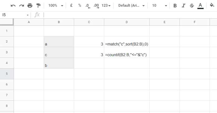
=MATCH("C", SORT({"A"; "C"; "B"}), 0)

Result: 3

=COUNTIF({"A"; "C"; "B"}, "<"&"C") + 1

Result: 3

Explanation of These Formulas

MATCH Formula:
- The MATCH function finds “C” in the sorted array {"A"; "B"; "C"}.
- It returns the relative position of “C” in the sorted list (which is 3).
- Syntax: MATCH(search_key, range, [search_type])
- Set search_type to 0 for an exact match. Otherwise, if there are duplicates, the formula may return the position of the last occurrence.
COUNTIF Formula:
- Syntax: COUNTIF(range, criterion)
- COUNTIF({"A"; "C"; "B"}, "<"&"C") + 1 counts how many values are smaller than “C” in the list, then adds 1 to determine the rank.

How to Replace the Array with a Cell Range

Instead of using an array like {"A"; "C"; "B"}, we can replace it with a cell range as follows:

=MATCH("C", SORT(B2:B), 0)
=COUNTIF(B2:B, "<"&"C") + 1

Rank data in Google Sheets by alphabetical order using formulas

This allows us to dynamically rank data by alphabetical order in Google Sheets based on the values in column B.

Rank an Entire Column Alphabetically

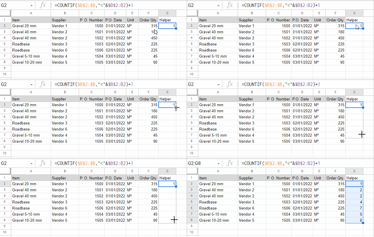
Let’s say we have text values in column B (B2:B8) and want to rank them alphabetically.

Non-Array Formula (Drag Down)

Insert the following formula in G2 and drag it down to G8:

=COUNTIF($B$2:$B, "<"&$B2) + 1

$B$2:$B is an absolute reference to fix the range.
"<"&$B2 dynamically compares each value in column B.

Rank all text values in a column alphabetically

Alternatively, using MATCH:

=MATCH(B2, SORT($B$2:$B), 0)

SORT($B$2:$B) sorts the column alphabetically.
MATCH(B2, …, 0) finds the position of each text value in the sorted list.

Using an Array Formula for Google Sheets Alphabetical Ranking

Instead of dragging down formulas, we can use an array formula to rank all values at once.

Insert this formula in G1:

={"Rank"; ArrayFormula(IF(B2:B="", , COUNTIF(B2:B, "<"&B2:B) + 1))}

={"Rank"; IFNA(ArrayFormula(MATCH(B2:B, SORT(B2:B), 0)))}

This formula ranks all text values in column B automatically.

Conclusion

The RANK function doesn’t support text, but using MATCH or COUNTIF, we can easily rank text in Google Sheets. These methods allow you to rank individual values or entire columns for use in Pivot Tables or sorting operations.

That’s all about how to rank data by alphabetical order in Google Sheets!