The PRODUCT function itself is an array formula. It takes arrays (cell ranges) and returns a single-cell result. So we can’t use it as an array formula to calculate row-wise products in Google Sheets.
When you want to multiply a series of numbers together row-wise, either you may depend on a drag-and-drop PRODUCT formula or an alternative array formula.
The alternative to the Product array formula can be a dynamic formula using a QUERY combo formula or using a non-dynamic formula that uses the asterisk (*) operator.
To make you understand why the Query or asterisk is a must for calculating row-wise products, please see the below example.
Update:- We can make the Product an array formula by using BYROW or BYCOL functions depending on the data orientation. I’ve updated this post to include that formula.
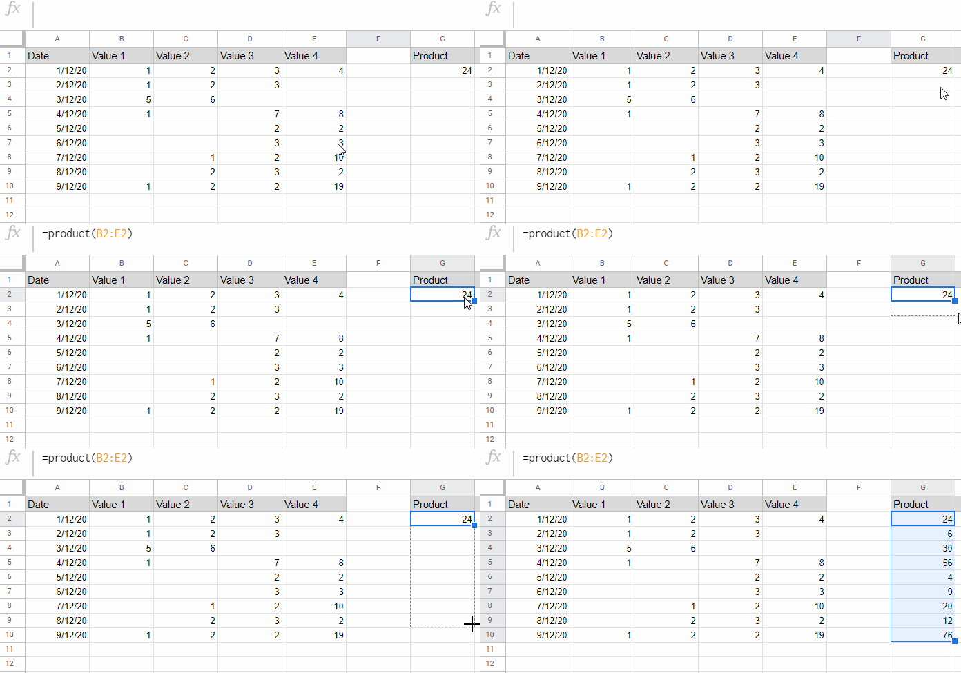
Drag-and-Drop Formula:

In the above example, I have used the Product formula in cell G2 and dragged it down to cover all the rows.
In this tutorial, I am talking about three array formula alternatives to the above Product non-array formula.
Among the three solutions for the row-wise products in Google Sheets, the simplest solution is using the asterisk and Byrow. But the former is not a dynamic formula.
Row-Wise Products Using Asterisk in Google Sheets (Non-Dynamic)
If the number of columns is limited as above, we can use the asterisk as below for row-wise products in Google Sheets.
Some of you may think that you can use the asterisk operator-based formula as below.
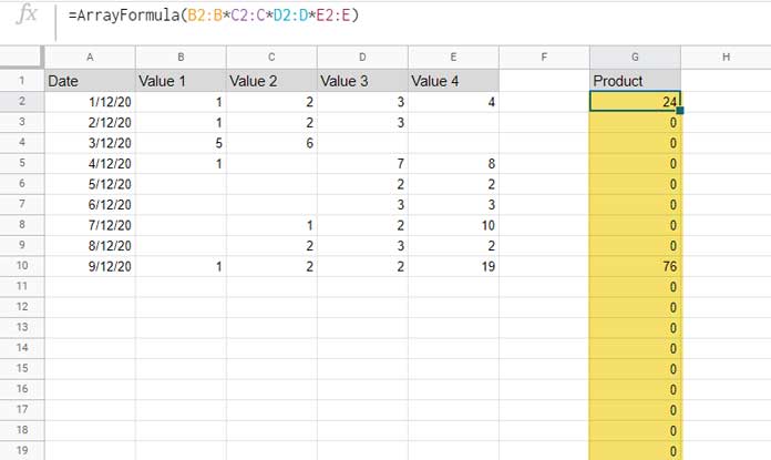
=ArrayFormula(B2:B*C2:C*D2:D*E2:E)But it is not correct!
It would return 0 in some cells in the result column. Also, you can see that several 0’s are like a trail in the entire column after the last row (row # 10).

When you multiply a number >0 with zero or zero with a number >0, the result will be 0.
Since the formula treats the values in the blank cells as zeros, the above-said issue arises.
Solutions to Correct the ‘Error’
To make this formula work correctly, we should specify two things in the formula. In the below steps, I am going to explain them.
1. Replace blank cells in the range with the number 1 in the formula expression itself.
2. Limit the formula to expand only up to the last non-blank cell in column A.
How to implement the above two points in the formula and return the correct row-wise products by using the PRODUCT array formula alternative in Google Sheets?
We can use a bunch of IF logical tests with every column as below.
Formula 1:
=ArrayFormula(
     if(B2:B="",1,B2:B)*
     if(C2:C="",1,C2:C)*
     if(D2:D="",1,D2:D)*
     if(E2:E="",1,E2:E)
)
The above formula in cell G2 would return the correct row-wise products in Google Sheets but would leave the number 1, instead of 0, in the blank rows.
Now we have to remove the # 1 by limiting the formula to expand until the last row with value.
Here is that one.
Formula 2:
=ArrayFormula(
     if(
        A2:A="",,
        if(B2:B="",1,B2:B)*
        if(C2:C="",1,C2:C)*
        if(D2:D="",1,D2:D)*
        if(E2:E="",1,E2:E)
     )
)
The above formula is the alternative to the Product array formula in Google Sheets.
I am not recommending the above formula in the following two scenarios.
1. If there are several columns, writing the formula without errors may be a difficult task.
2. When you insert new columns between the existing columns, you may want to edit the formula manually. So time taking and error-prone.
PRODUCT Array Formula Alternative Using Query Combo (Dynamic)
The formula that you are going to get here will help you overcome the above drawbacks.
First of all, let’s see how we can write a formula to replace formulas # 1 and # 2 above.
The following Query in cell G1 will replace formula # 1 and the subsequent Query and IF combo will replace formula # 2.
Formula 3 (Replaces Formula 1):
=ArrayFormula(query({if(B2:E="",1,B2:E)},"Select Col1*Col2*Col3*Col4",0))Formula 4 (Replaces Formula 2):
=ArrayFormula(if(len(A1:A),query({if(B2:E="",1,B2:E)},"Select Col1*Col2*Col3*Col4",0),))Note:- Please insert the above formulas (either of the one) in cell G1 as it returns a header other than products.
The above formulas, Formula 1 and Formula 3 are the wrong formulas and whereas Formula # 2 and Formula # 4 are the correct non-dynamic formulas to return the row-wise products in Google Sheets.
We can modify formula # 4 as an alternative to the dynamic PRODUCT array formula for row-wise products in Google Sheets.
Important Notes:-
Formula 2 and Formula 4 are not dynamic and behave differently when you insert new columns. You should edit both formulas when you insert new columns.
For example, I have inserted a new column after column C. The changes in the formulas will be as follows (please pay attention to the bold part).
In Formula # 2;
if(B2:B=””,1,B2:B)* if(C2:C=””,1,C2:C)* if(D2:D=””,1,D2:D)* if(E2:E=””,1,E2:E)* if(F2:F=””,1,F2:F)
In Formula # 4;
Select Col1*Col2*Col3*Col4*Col5
Here is a dynamic product array formula alternative for row-wise products. You can include several columns in this, and insert new columns that will be auto-added to the formula.
Formula 5:
={"Product";
     ArrayFormula(
        if(
           len(A2:A),
              Query(
                 query(
                    ({if(B2:E100="",1,B2:E100)}),"Select "&"Col"&TEXTJOIN("*Col",1,COLUMN(B1:E1)-1)
                 ),
                 "offset 1",0
              ),
        )
     )
}
Formula Explanation
Let’s peel away the inner Query (which is a modified version of Formula # 4) and learn that first.
=ArrayFormula(
     query(
        ({if(B2:E100="",1,B2:E100)}),"Select "&"Col"&TEXTJOIN("*Col",1,COLUMN(B1:E1)-1)
     )
)
In this, the SELECT clause in Formula 4, i.e., Select Col1*Col2*Col3*Col4, replaced by a dynamic column reference, i.e., Select "&"Col"&TEXTJOIN("*Col",1,COLUMN(B1:E1)-1).
You May Like: What is the Correct Clause Order in Google Sheets Query?
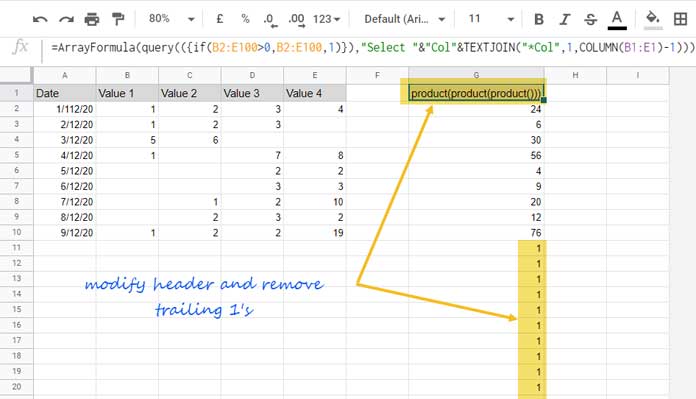
I will explain it. Before that, please see the result returned by the above formula.

Now to the explanation.
The formula COLUMN(B1:E1)-1 returns the numbers 1,2,3, and 4.
The column numbers of the range B1:E1 (the columns involved in the Product calculation) are 2, 3, 4, and 5. To make it 1, 2, 3, and 4, I have used -1.
The TEXTJOIN converts the numbers to Col1*Col2*Col3*Col4 (Query syntax).
It is dynamic because when you insert new columns in the range B2:E, the column reference inside the COLUMN will be adjusted accordingly.
What’s the role of the outer Query in the final row-wise product’s formula?
It’s actually for offsetting 1 row (see G1 in the image above) to remove the header.
After removing the header, we have added a custom header using Curly Braces as per the below syntax.
{"Product";Query_Formula}You can change the text as per your wish.
PRODUCT Array (Spill Down) Formula Using BYROW – New
I’ve used column A (which contains dates) to limit the expansion of the array in blank rows in the above two product array formulas (asterisk and query).
But if you use the following Product and Byrow in cell G1, you can avoid using that column.
={"Product (Byrow)";byrow(B2:E,lambda(row,if(count(row)=0,,product(row))))}Because the formula counts the number of values in each row, and if it’s 0, it returns a blank else product.
I’ve added the above formula in cell H1 in the sample sheet below.
That’s all about the alternative to the PRODUCT array formula for row-wise products in Google Sheets.
Thanks for the stay. Enjoy!
Resources:


