Let’s see how to populate a full (entire) month’s dates based on a drop-down in Google Sheets. We will use an array formula for this.

For recording monthly attendance of employees, you may want to get an entire month’s dates based on a drop-down.

I know your requirements may be entirely different.

Whatever the reason, you can depend on my formula if you want an entire month’s calendar, either in a row or column.

It’s common practice to select a year and then a month from drop-downs and populate the dates that fall in that month and year in a row or column.

I have seen Google Sheets users using different approaches to get this result.

I have an array formula that does this job brilliantly. No matter which month and year, it works flawlessly. Before going to that, see how it works.

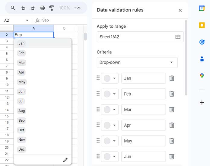
In this example, I have only created the drop-down for the month (A2). The year is in cell A1.

I keyed the same formula in cells B2 and B3, which populates the selected month’s full dates.

But I’ve formatted the dates as days of the week in one row and sequence numbers in another row.

How to Populate a Full Month’s Dates Based on a Drop-Down in Google Sheets

Let’s begin with creating the drop-down in cell A2.

Steps:

In cell A2, go to the menu Data > Data validation and create a drop-down menu containing month names as menu items.

If you find any issues, please check this tutorial: The Best Data Validation Examples in Google Sheets.

Your drop-down menu to select the month to populate the corresponding dates is ready.

You can create another drop-down menu in cell A1 containing the years to select. But I am leaving that part. I prefer to hand-enter the year in cell A1.

You can use the below formula in both cells B2 and B3 to populate an entire month’s dates based on the year entered in cell A1 and the month selected in cell A2.

=LET(dt,DATE(A1,MONTH(A2&1),1),IF(LEN(A1),SEQUENCE(1,EOMONTH(dt,0)-dt+1,dt),))

The output will be date values.

You can select the formula results and apply the Format menu > Number > Date to convert them to dates. But we want different formatting.

Let’s see how to do that.

Tip:

Want the result in a column? Just wrap the formula within TOCOL like =TOCOL(above_formula).

Formatting: Date to Day of the Week and Number

First, Select the range B2:AF2.

Go to the Format menu > Number > Custom number format.

Enter ddd in the provided field and Apply.

Then select the range B3:AF3. There, enter dd in the custom number format field. That’s all that you want to do.

This way, you can populate a full (entire) month’s dates based on a drop-down in Google Sheets and format that to your requirements.

Anatomy of the Formula that Populates an Entire Month’s Dates in a Row

Here is the main part of the formula, which returns the start date of the month and year entered/selected in A1:A2.

Formula: DATE(A1,MONTH(A2&1),1)

Syntax: DATE(year, month, day)

We have a year in A1 and a month text in A2. We converted that month text to a month number using MONTH(A2&1).

If the entered year is 2023 and the month is February, the formula will return 1/2/2023 (DD/MM/YYY).

The role of LET is to assign dt, a name, to this formula so that we can use this name later part instead of the formula itself. It improves performance.

We have learned up to the below part.

LET(dt,DATE(A1,MONTH(A2&1),1),

We have used this date (dt name) in SEQUENCE to generate an entire month’s date based on the drop-down selection in cell A2 and the value in cell A1. Let’s see how.

Formula: SEQUENCE(1,EOMONTH(dt,0)-dt+1,dt)

Syntax: SEQUENCE(rows, [columns], [start], [step])

Where;

rows: 1 (we want sequence numbers [dates] in one row).

columns: EOMONTH(dt,0)-dt+1 (last date – first date in the month + 1, i.e., total days in the selected month and year).

start: dt (first date of the month)

The other parts of the formula are optional.