If you have employees working on an hourly basis, calculating payroll hours is easy in spreadsheet applications such as Google Sheets.
From a start time and end time, you can easily calculate their working hours.
By subtracting the start time from the end time, you can determine the duration of their shift in Google Sheets.
How is this possible?
Google Sheets stores dates and times as a single serial number. The integer part represents the day, and the decimal part represents the time.
The serial number represents the number of days since 1899-12-30, plus a decimal value representing the time of day.
Before proceeding to payroll hours calculation, one more thing:
If your employees’ working hours span two days, such as a night shift that starts on one day and ends on the next, I suggest you enter their start datetime and end datetime rather than just the time in and time out.
For example, if an employee starts working at 22:00:00 and ends their work at 02:00:00 the next day, it should be entered as 2024-06-11 22:00:00 (start) and 2024-06-12 02:00:00 (end). Otherwise, subtracting the start time from the end time can result in negative numbers, which will cause errors in the payroll calculation.
To format dates and times correctly in Google Sheets, use the format YYYY-MM-DD HH:MM:SS.
Ensuring accurate payroll hours calculation is important for both legal and operational reasons. Inaccurate calculations can lead to labor law violations, employee dissatisfaction, and potential lawsuits.
Sample Data and Expected Output
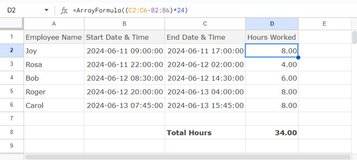
My sample data consists of employee names in column A, and their start datetimes and end datetimes in columns B and C.
In the table below, you can see my expected result in the fourth column.
| Employee Name | Start Date & Time | End Date & Time | Hours Worked |
| Joy | 2024-06-11 09:00:00 | 2024-06-11 17:00:00 | 8 |
| Rosa | 2024-06-11 22:00:00 | 2024-06-12 02:00:00 | 4 |
| Bob | 2024-06-12 08:30:00 | 2024-06-12 14:30:00 | 6 |
| Roger | 2024-06-12 20:00:00 | 2024-06-13 04:00:00 | 8 |
| Carol | 2024-06-13 07:45:00 | 2024-06-13 15:45:00 | 8 |
I have used datetime instead of time since their work spans two days. This is the best approach whether the start datetime and end datetime fall on the same day or not.
If your employees’ work hours always fall within a single day, you can use just time entries (without dates) to save ink when printing.
Let’s move to the formula to calculate the payroll working hours in Google Sheets.
Array Formula for Payroll Hours Calculation in Google Sheets
The generic formula to calculate payroll hours in Google Sheets is as follows:
=ArrayFormula((end_datetime-start_datetime)*24)Why do we multiply the difference between the start time and end time by 24?
It’s because the difference will be in the number of days due to the way Google Sheets stores datetime values, as mentioned earlier.
To convert this difference to actual hours, you multiply by 24 because there are 24 hours in a day.
In our table, the end_datetime is in cells C2:C6 and start_datetime is in cells B2:B6. So, you can use the following formula in cell D2 to calculate the payroll hours:
=ArrayFormula((C2:C6-B2:B6)*24)
Calculate Payroll Hours Only When Both Start and End Times Are Present
The above formula works well when both times are there. It shows 0 if both are missing, but gives wrong results if only one is missing.
This discrepancy arises because an empty cell value is interpreted as 0 (zero), corresponding to the date and time 1899-12-30 00:00:00.
If you want to resolve this issue, use the following generic formula instead of the previous one:
=ArrayFormula(
   IFERROR(
      IF(
         DATEVALUE(start_datetime)*DATEVALUE(end_datetime)>=0,
         (end_datetime-start_datetime)*24
      ), 0
   )
)
Let me explain this first, then we will proceed to the formula.
The DATEVALUE function returns a date value when a datetime is present, otherwise, it returns an error.
This means if DATEVALUE(start_datetime) * DATEVALUE(end_datetime) outputs a number, both start and end times are present.
We have used the IF function to incorporate this capability into the payroll hour calculation formula. The syntax is:
IF(logical_expression, value_if_true, value_if_false)Where:
logical_expression:DATEVALUE(start_datetime) * DATEVALUE(end_datetime)>=0value_if_true:(end_datetime - start_datetime) * 24value_if_false: Omitted
The formula will return a #VALUE! error when either of the times is empty due to the use of DATEVALUE. The IFERROR function is used to return 0 instead of the error value.
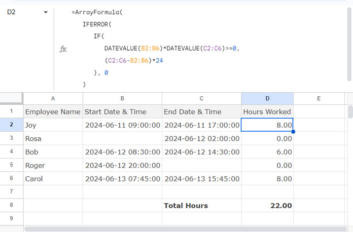
Here is the formula:
=ArrayFormula(
   IFERROR(
      IF(
         DATEVALUE(B2:B6)*DATEVALUE(C2:C6)>=0,
         (C2:C6-B2:B6)*24
      ), 0
   )
)
Since there’s missing data (empty time) in rows #3 and #5, the formula returns 0.00 for those rows.
Resources
Here are some Google Sheets resources specifically for start-time and end-time calculations.


Thank you! This helped a lot and saved me a bunch of trial and error. I had no idea about the array formula feature.
I am a rideshare driver. I record the time I start and the time I end.
I want to know how many hrs/minutes per ride.
For example, if I work 9 hours, 30 minutes, and give 22 rides, how do I determine how much time each ride took?
Hi, Bond,
It is not possible to code a formula without seeing the data formatting.
Can you please make a copy of your sheet and share it (the URL) after replacing the original data with mockup data?
You can leave it in “reply” below. I won’t publish it.
Hello,
I have the format in 24hr time and I get an error message when the end time gets to midnight. An example is 17:30 – 00:03, the error message that pops up is: Error
Function HOUR parameter 1 value is negative. It should be positive or zero.
I have it set up exactly how you show in the examples, conversion of hours, minutes, etc.
Hi, Natalie,
In such a case, if you want to use the same formula, use DateTime (Timestamp);
Start: 16/01/2020 17:30:00
End: 17/01/2020 00:30:00
…instead of time.
Note: Use the DateTime format as per your Locale.
Also, there is a different method using a ‘new’ formula. See the link to that guide at the bottom of my post (the second link under “Additional Resources”)
Using the 12-hour clock format, what if the shift duration starts at PM and ends at AM?
I am having trouble setting up a calculation sheet on Google Docs. For example, how would you formulate the durations of hours from 3:00 PM to 12:30 AM on a Google Doc?
Hi, Brenda,
You can refer to the tutorial under “Additional Resources” above (Point # 2).
Assume cell F3 contains 3:00 pm (15:00:00) and F4 contains 12:30 am (00:30:00). That means the job starts on Day 1 and ends on Day 2.
In such scenarios, to find the duration use this formula.
=MOD(F4 - F3,1)Format the output to Duration from the Format menu, Number.
Best,
How to take a break in to your calculation?
Hi, Michel,
Please check the following tutorial.
1. How to Deduct Lunch Break Time From Total Hours in Google Sheets.
Check this too.
2. Google Sheets: The Best Overtime Calculation Formula.
Best