One Filter Function as the Criteria in Another Filter Function in Google Sheets

Published on

We can use one filter function output as the criteria/condition in another filter function in Google Sheets.

If the filter function result, which is in use as the criteria in another, is a single value, you won’t face any issue in such use.

But in the case of multiple values in the filter formula result, then there is a different approach in the criteria use!

With a detailed example, we can learn how to use a filter function output as the criteria in another filter function in Google Sheets.

How to Use Filter Function Output as the Criteria in Another Filter Function in Google Sheets

Filtering a dataset (small or large) is possible using different methods in Google Sheets. For this, we can use two menu commands as well as two functions.

What are they?

  1. The menu commands (menu options) to Filter data sets in Google Sheets are Slicer and Create a filter. Both are available under the Data menu in Sheets.
  2. The said two functions are Query and Filter. The Query is more advanced and better than the Filter function.

Learning Query is a must to handle large datasets effortlessly. But wherever possible, use the Filter function as it’s said to be more resource-friendly in Sheets.

Let’s back to the problem to solve or scenario.

I have two tables. One contains a list of fruits and their quantity. Let us call this table, Table 1.

The second table, called Table 2, contains the same list (but unique fruits only). Instead of quantity, it contains the unit price.

I want to filter Table 1 based on Table 2. I mean filter the fruits in Table 1 if their unit price in Table 2 is, for example, less than a particular value, for example, <5.

That means first we need to filter the second table with the criteria, i.e. unit rate <5.

If the filter returns only one fruit name, then there is no issue in using it as the condition in the second filter formula that filters Table 1. Else we must use JOIN/TEXTJOIN and REGEXMATCH together with.

All these I am going to detail below. Before that see those two tables.

Table 1 and 2:

Sample Tables 1 and 2 for Filtering in Sheets

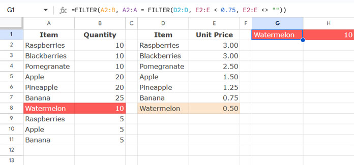
Filter within Filter in Google Sheets – Single Condition

How to filter the fruits in Table 1 of which the unit price is <2 in Table 2?

When you check the unit price (column E) in Table 2, you can find that there is only one fruit coming in that price range, i.e. “watermelon”.

Formula # 1:

=filter(A3:B,A3:A="watermelon")

The above formula will filter Table 1 if the rows in the range A3:A matches “watermelon”

In the above formula “watermelon” is the criterion/condition. We can replace that with another filter formula.

The following formula will fetch the item “watermelon” from Table 2 as it is the only item with the unit price <2.

Formula # 2:

=filter(D3:D9,E3:E9<2)

That means, we can replace the criterion “watermelon” in Filter Formula # 1 as below.

Formula # 3:

=filter(A3:B,A3:A=filter(D3:D9,E3:E9<2))

The above is one basic example of using filter function output as the criterion/condition in another filter function in Google Sheets.

Point to be Noted

In the above filter formula (Formula # 3), you may have noticed that I have used a closed range in the inner filter. Let’s make that an open range.

Change D3:D9 and E3:E9 with D3:D and E3:E respectively.

Formula # 4:

=filter(A3:B,A3:A=filter(D3:D,E3:E<2))

The above formula will then return a blank output!

The reason is, the inner filter formula not only returns “watermelon” but also returns some blank cells because of the use of the open (infinite) ranges.

In such a case, I mean using one filter function output as the criteria in another filter function, refine the inner filter output to exclude blanks. How?

Use the below filter, which filters out blanks, as the criteria.

Formula # 5:

=filter(D3:D,(E3:E<2)*(E3:E<>""))

So the final formula will be;

Formula # 6:

=filter(A3:B,A3:A=filter(D3:D,(E3:E<2)*(E3:E<>"")))
One Filter as Criteria in Another Filter - Single Criterion

Filter within Filter in Google Sheets – Multiple Condition

Just change the criterion in the inner Filter formula to <5.

Formula # 7:

=filter(D3:D,(E3:E<5)*(E3:E<>""))

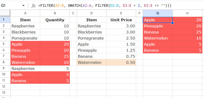
It would return the fruits “apple”, “pineapple”, “banana”, and “watermelon”. These are the conditions to filter Table 1.

But the above filter formula as the criteria in another filter as earlier would return an #N/A! error.

Formula # 8:

=filter(A3:B,A3:A=filter(D3:D,(E3:E<5)*(E3:E<>"")))

Here, to use one filter function result as the criteria in another filter function we can make use of the REGEXMATCH and JOIN function in Google Sheets.

Must Read: Regexmatch in Filter Criteria in Google Sheets [Examples].

It’s similar to the use of the IN operator (alternative) in Query.

Related: The Alternative to SQL IN Operator in Google Sheets Query (Also Not IN).

Steps

Use the JOIN function to combine the multiple criteria (Formula # 7) as below.

Formula # 9:

=join("|",filter(D3:D,(E3:E<5)*(E3:E<>"")))

Alternatively, if you like, you can also use it as below.

=textjoin("|",true,FILTER(D3:D,E3:E<5))

In the first formula (JOIN based), the Filter function itself excludes blank cells from the output. But in the second one (TEXTJOIN based), the Textjoin removes blanks. I prefer the second formula.

Replace A3:A=filter(D3:D,(E3:E<5)*(E3:E<>"")) in Formula # 8 with =REGEXMATCH(A3:A,textjoin("|",true,FILTER(D3:D,E3:E<5)))

So the final formula would be;

Formula # 10:

=filter(A3:B,REGEXMATCH(A3:A,textjoin("|",true,FILTER(D3:D,E3:E<5))))
One Filter as Criteria in Another Filter - Multiple Criteria

That’s all about how to use one filter formula as the criteria in another filter formula in Google Sheets. Thanks for the stay, enjoy!

Resources

Prashanth KV
Prashanth KV
Your Trusted Google Sheets and Excel Guide Prashanth KV brings a wealth of experience in Google Sheets and Excel, cultivated through years of work with multinational corporations in Mumbai and Dubai. As a recognized Google Product Expert in Docs Editors, Prashanth shares his expertise through insightful blogging since 2012. Explore his blog for practical tips and guidance on maximizing your spreadsheet skills.

Hierarchical Numbering Sequences in Excel

Creating hierarchical numbering sequences in an Excel spreadsheet can significantly improve the way you...

How to Easily Repeat a Sequence of Numbers in Excel

Excel offers multiple ways to accomplish tasks, and the simplicity of each approach depends...

Create a Sequence of Dates at Every Nth Row in Excel (Dynamic Array)

Would you like to create a sequence of dates in every nth row in...

XMATCH Row by Row: Finding Values Across a Range in Google Sheets

Using the BYROW function with XMATCH in Google Sheets allows us to match values...

More like this

XMATCH Row by Row: Finding Values Across a Range in Google Sheets

Using the BYROW function with XMATCH in Google Sheets allows us to match values...

Limit Formula Expansion to a Specific Row in Google Sheets

In this tutorial, I’ll explain how to limit the expansion of an array formula...

3-D Referencing Structured Data Tables in Google Sheets

When you have several tables within a single sheet—not across multiple sheets in a...

LEAVE A REPLY

Please enter your comment!
Please enter your name here

This site uses Akismet to reduce spam. Learn how your comment data is processed.