There are two functions to raise a number to a power in Google Sheets: POWER() and POW(). In addition to these functions, the caret symbol ^ can also be used for exponentiation.

While POWER() is categorized as a Math function in Google Sheets, POW() appears under the Operator category.

Let me show you how to raise a number to a power in Google Sheets using both functions and the caret symbol.

Note: The POW function may have been introduced in earlier versions of Google Sheets, while POWER was added later for compatibility and better readability.

How to Raise a Number to a Power in Google Sheets

You can use the POWER(), POW(), or caret (^) operator to return a base number raised to an exponent.

When you’re raising a number to a power, you’re essentially multiplying that number (the base) by itself repeatedly—the number of times specified by the exponent.

Raise a Number to a Power Using the POWER() Function

Syntax:

POWER(base, exponent)

Example:

=POWER(10, 3)

The result is 1000, which is equivalent to:

=10*10*10

Raise a Number to a Power Using the POW() Function

You can get the same result using the POW() function in Google Sheets. Both POWER() and POW() work the same way in Sheets.

As far as I know, Excel only supports the POWER() function and does not recognize POW().

Syntax:

POW(base, exponent)

Example:

=POW(10, 3)

Raise a Number to a Power Using the Caret (^)

The caret operator works in both Excel and Google Sheets. You can raise a number to a power like this:

=10^3

This also returns 1000.

These are the three ways to raise a number to a power in Google Sheets.

Points to Note

All three methods—the POWER() function, POW() function, and caret operator—work with arrays. Here’s an example using ARRAYFORMULA:

Raise a Range of Numbers to a Power in Google Sheets

=ARRAYFORMULA(A2:A5^3)

You can also specify both base and exponent as arrays:

=ARRAYFORMULA(B2:B6^C2:C6)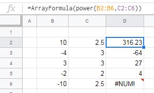

Negative Numbers as Base

When using a negative base, the exponent must be an integer. Otherwise, the formula will return a #NUM! error saying: “POWER evaluates to an imaginary number”

This is a known behavior in Google Sheets.

Bonus Tip: Use of Power, Pow, or ^ in Other Formulas

I often use the caret in formulas like QUERY, ARRAY_CONSTRAIN, and SORTN when I want the formula to return all rows.

Sometimes, it’s not practical to specify the number of rows you want to return after filtering or sorting. In those cases, I use a trick with the power operator.

Example: Caret in SORTN

Here’s an example using SORTN to return a sorted list of unique values:

=SORTN(A2:A, 9^9, 0, 1, TRUE)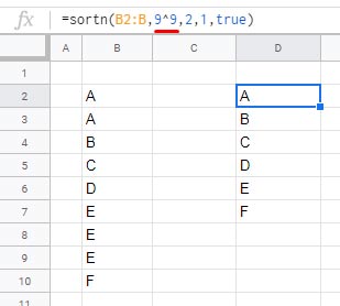

In this case, 9^9 represents a large number to effectively say “return all rows.”

That’s how you can raise a number to a power in Google Sheets using POWER(), POW(), or ^.