Sum Multiple Sum Columns in DSUM – Google Sheets Guide

To sum multiple sum columns in DSUM, you can combine it with SUMPRODUCT in Google Sheets. This method offers an advantage over SUMIFS, allowing you to apply multiple criteria while summing multiple columns dynamically.

The key is to specify the columns to sum as an array and wrap DSUM inside SUMPRODUCT.

Generic Formula

=SUMPRODUCT(DSUM(A1:D, {"field 1", "field 2", "field 3", ...}, F1:F2))

Where:

A1:D: Data range
{“field 1”, “field 2”, “field 3”, …}: Field labels of the columns to sum
F1:F2: Criteria range

Example: Summing Multiple Sum Columns in DSUM

Sample Data

The dataset includes student names (Column A) and their marks in three subjects (Columns B–D).

Name	Maths	Physics	Chemistry
Rose	90	86	90
Rose	94	80	89
Rose	96	79	91
Mike	98	89	75
Mike	97	82	78
Mike	98	84	89

We will sum the total marks of “Rose” in all three subjects.

Step-by-Step Guide

1. Define the Criteria

Enter “Name” in F1 (criteria label).
Enter “Rose” in F2 (criteria value).

2. Enter the DSUM Formula

In H2, enter:

=SUMPRODUCT(DSUM(A1:D, {"Maths", "Physics", "Chemistry"}, F1:F2))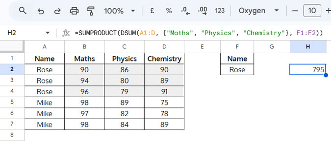

Example of Summing Multiple Columns in DSUM

Alternative Approach: Using Column Numbers

Instead of using column names, you can refer to the column positions:

=SUMPRODUCT(DSUM(A1:D, {2, 3, 4}, F1:F2))

How the Formula Works

1. DSUM with Multiple Sum Columns

When specifying multiple sum columns like {“Maths”, “Physics”, “Chemistry”} or {2, 3, 4}, DSUM returns separate totals for each column.

However, DSUM alone does not sum them together, so we wrap it inside SUMPRODUCT.

2. Why Use SUMPRODUCT Instead of SUM?

While you can use SUM with ARRAYFORMULA, SUMPRODUCT simplifies the formula:

=SUM(ARRAYFORMULA(DSUM(A1:D, {2, 3, 4}, F1:F2)))

Can be replaced with:

=SUMPRODUCT(DSUM(A1:D, {2, 3, 4}, F1:F2))

Key Benefits:

Shorter & cleaner formula
No need for ARRAYFORMULA
Handles arrays efficiently

Dynamic Approach: Sum Multiple Columns in DSUM with SEQUENCE

If you have several continuous columns to sum, manually listing them can be tedious. Instead, use the SEQUENCE function to generate field numbers dynamically.

Formula Using SEQUENCE

=SUMPRODUCT(DSUM(A1:D, SEQUENCE(3, 1, 2), F1:F2))

How It Works

SEQUENCE(3, 1, 2) generates {2, 3, 4} dynamically.
The formula sums 3 continuous columns starting from the 2nd column (Maths).

Adjusting for More Columns:

Change 3 to the total number of columns, and 2 to the first column’s position.

Conclusion

By using SUMPRODUCT with DSUM, you can efficiently sum multiple sum columns in DSUM while applying criteria dynamically.

Key Takeaways:

Use column labels or numbers in DSUM
Wrap DSUM in SUMPRODUCT for correct totals
Use SEQUENCE for dynamic column selection

This method is powerful for conditional summing across multiple columns in Google Sheets.