The MROUND function in Google Sheets is a useful mathematical function that rounds a number to the nearest integer multiple of another number. This tutorial will explain how to use the MROUND function and highlight its differences from the ROUND function.
Purpose of the MROUND Function
The purpose of MROUND is to round a given number (known as “value”) to the nearest integer multiple of another number (called “factor”).
MROUND Function – Syntax and Arguments
Syntax:
MROUND(value, factor)Arguments:
- value: The number you want to round.
- factor: The number to which you want to round the value. Both arguments are required; omitting the factor will result in a #N/A error.
Examples
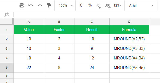
In the following examples, the formulas round the values in column A (cell range A2:A5) to the nearest integer multiples of the values (factor) in column B (cell range B2:B5).

For example, let’s look at row 5, where the value is 22 (in cell A5) and the factor is 8 (in cell B5).
To find the nearest integer multiple of 8, consider the following multiples:
- 1 x 8 = 8
- 2 x 8 =16
- 3 x 8 = 24
The integer multiples of 8 are 8, 16, and 24. In this case, the nearest integer multiple of 22 (A5) is 24. Thus, the formula in cell C5 returns:
=MROUND(A5, B5)Result: 24
This example illustrates how the MROUND function works effectively.
Comparing MROUND with ROUND in Google Sheets
Both MROUND and ROUND are mathematical functions in Google Sheets, but their purposes differ significantly.
- The ROUND function rounds a number to a specified number of decimal places according to standard rounding rules.
Example 1:
=ROUND(22.1254, 2)Result: 22.13
Example 2:
=ROUND(22.1254, 1)Result: 22.1
In contrast to ROUND, the MROUND function focuses on rounding to integer multiples rather than decimal places.
Conclusion
Understanding how to use the MROUND function can greatly enhance your data manipulation capabilities in Google Sheets. Whether rounding numbers to meet specific criteria or comparing them to the ROUND function, knowing the distinctions will help you apply these functions effectively in your spreadsheets.


