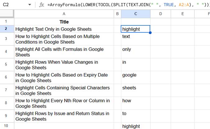
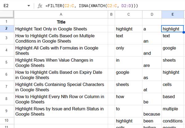
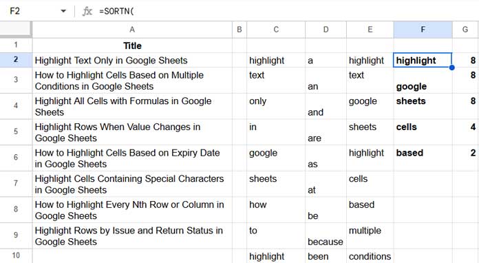
As an SEO, sometimes you may require to find the most frequent keywords from a list of titles. For this, you can use Google Sheets.

Of course, there is no built-in formula for this. I don’t know about the add-on availability. But I have written two formulas that you may find useful.

I’ve two types of solutions (formulas) as I’m approaching the topic from two different angles – single-word keywords and multiple word keywords.

In the first case (single word keywords), you can make use of the different clauses in the Query function to find the most 10 or ‘n’ frequent keywords from a list of post titles in a column in Google Sheets.

In the second case (multiple word keywords), things are quite different. Here, in addition to the post titles as a list, you should also specify the keywords as another list.

The formula would return the count of that specified keywords.

To get the most frequent keywords from post titles in Google Sheets, in both the above cases, as I have mentioned, I’ll use the Query function. But we may also require to use some other functions with the Query.

How to Get the Most Frequent Keywords from Post Titles in Google Sheets

For every formula explanation, we may require sample data. Here I am going to use a few of the post titles from my own blog.

My post titles comply with the following.

• There should not be any open or close brackets in the titles.
  • I mean the post titles should exclude () (parenthesis), {} (curly brackets), [] (square brackets), and <> (angle brackets).
  • If you have such brackets in your titles, do replace them with the Edit > Find and replace command (menu item) in Google Sheets.
• The above points are only applicable to the second case, i.e. in finding the frequency of given multiple word keywords.

Here are the titles from which we are going to find the most frequent keywords in Google Sheets.

Single Word Keywords

Get my formula first and then read the formula explanation. The following Query formula is for inserting in cell B1 in the sheet that contains the above list.

Formula:

=Query(
     transpose(
        split(
           query(A2:A100,,9^9)
           ," ")
     ),
     "Select Col1,
     Count(Col1) 
     where not Col1 matches 'a|an|and|as|or|where|if|in|how|by|all|for|to|use|of|the|with' 
     group by Col1 
     order by Count(Col1) desc",0
)

Formula Explanation:

The formula query(A2:A100,,9^9) combines the post titles into a single cell. This way we can avoid the use of the functions Join or TextJoin.

The Split function splits this Query result based on space as the delimiter. So we will get a row with several words in each cell in that row.

The Transpose function changes the orientation of the Split result. So the data will be now in a single column.

The outer Query groups this column. The concerned two clauses in the formula are Select Col1 and group by Col1.

We have used the aggregation function Count as what we want to get is the most frequent keywords from titles.

I have used the Matches clause where not Col1 matches 'a|an|and|as|or|where|if|in|how|by|all|for|to|use|of|the|with' to exclude certain keywords from the grouping (separated by the pipe signs). If you wish, you can include more or delete a few of them.

The formula part, i.e. order by Count(Col1) desc, is for sorting the count of the most frequent keywords in descending order.

If you want you can include the part limit 10 (which is not a part of the “Formula”) to get the top 10 most frequent keywords from post titles in Google Sheets.

That’s all.

Multiple Word Keywords (Keywords to be Specified Beforehand)

To get the frequency of multiple word keywords from titles in Google Sheets, other than the post titles, we should specify the keywords.

Please see the following screenshot.

Important Notes:

Here all the keywords contain two words each.

If you want to find the frequency of keywords containing 3 words, do not include them in the above list in C2:C. In that case C2:C must only contain keywords with 3 words.

That means the list in C2:C should only contain unique number word keywords.

In rare case, if a post title contains multiple word keywords that are adjoining, the formula may get only a near-perfect result.

For example, see the first post title query function in google sheets. In this “query function” and “google sheets” are two keywords.

But if the title is like this; query function in google sheets query function, there would be a problem as there are two adjoining keywords at the last.

In four steps (the fourth step is optional though), we can write the formula to get the count of most frequent multiple word keywords from titles in Google Sheets.

There are four formulas in each step. We will combine them in the final step. Here are those steps.

Step # 1 – Regex

In cell F2, insert the below Regexreplace formula to replace the multiple word keywords in the post titles with the regular expression (.*).

=ArrayFormula(REGEXREPLACE(A2:A100,textjoin("|",true,C2:C100),"(.*)"))

(you can see the result in step # 2 screenshot below)

Step # 2 – Regex

In cell G2 insert another Regexreplace formula.

=ARRAYFORMULA(IFNA(REGEXREPLACE(A2:A100,F2:F100,{"$1","$2","$3","$4"})))

The following formula part in the above formula makes the formula to return results in 4 columns (G, H, I, and J).

{"$1","$2","$3","$4"}

If your post title is long and contains more than 3 keywords (normally it may not), then you can increase the number of columns in the result by changing the above formula part as {"$1","$2","$3","$4","$5","$6"}.

This means the formula will extract a maximum number of six multiple word keywords from post titles in each row in Google Sheets.

In step # 3 below, we will get the most frequent (listed) multiple word keywords from titles in Google Sheets.

I have used the words ‘listed’ as we are using only the values (words) in the list C2:C for the count.

Step # 3 – Query

Let’s flatten the second formula output. So the multiple column output will be placed in a single column and so that we can Query that output.

In cell K2, key this formula in.

=query(
     flatten(G2:J100),
     "Select Col1,Count(Col1) where Col1 is not null group by Col1 order by Count(Col1) desc",0
)

You will get the below result in K2:L.

Step # 4 – Final Formula

Finally, in cell D2 use the below optional Vlookup. Yes, the below formula is optional as you can use step # 3 formula itself as the final formula.

=ArrayFormula(ifna(vlookup(C2:C5,K2:L6,2,0)))

Let’s combine all the formulas.

=ArrayFormula(ifna(vlookup(C2:C100,query(flatten(IFNA(REGEXREPLACE(A2:A100,REGEXREPLACE(A2:A100,textjoin("|",true,C2:C100),"(.*)"),{"$1","$2","$3","$4"}))),"Select Col1,Count(Col1) where Col1 is not null group by Col1 order by Count(Col1) desc",0),2,0)))

Just keep the D2 formula and delete all the formulas which we have inserted in other cells in the earlier steps.

That’s all about how to get the most frequent keywords from titles in Google Sheets.

Thanks for the stay. Enjoy!