The MMULT function in Google Sheets often results in a #VALUE! error when applied to infinite (open) ranges. This issue arises due to empty cells in either matrix1, matrix2, or both. Let’s first explore the root cause of this problem and then review two approaches to use MMULT effectively with infinite rows.

MMULT in Infinite Rows: Understanding the Issue of Empty Cells

In array formulas, we typically use open ranges to account for data growth. However, this creates a challenge with MMULT, as it cannot handle empty cells within the matrices. For example:

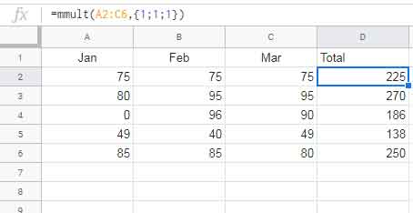
Closed Range Example

The following formula calculates row totals for the range A2:C6:

=MMULT(A2:C6, {1;1;1})

This works correctly because there are no empty cells in the range.

Open Range Example

Expanding the range to A2:C:

=MMULT(A2:C, {1;1;1})

results in a #VALUE! error. This occurs because MMULT treats naturally empty cells as invalid, even though they effectively have a value of 0.

Solutions to Use MMULT in Infinite Rows

Here are two methods to address this issue.

Approach 1: Convert Empty Cells to Zero

This approach replaces empty cells with 0, allowing MMULT to work with infinite rows. Then, a logical test ensures empty rows return blank results.

Step 1: Convert Empty Cells to Zero

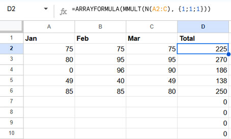
Use the N function to replace empty cells in matrix1 with 0:

=ARRAYFORMULA(MMULT(N(A2:C), {1;1;1}))

The N function is designed to convert blank cells to 0 while leaving numeric values unchanged. Since N is not inherently an array function, wrapping it with ARRAYFORMULA ensures that the entire range is processed correctly. This step ensures that the MMULT function can perform calculations without errors caused by blank cells.

Step 2: Replace Zeros with Blanks

Wrap the result in a LET function to clean up the output:

=ARRAYFORMULA(LET(result, MMULT(N(A2:C), {1;1;1}), IF(result=0, , result)))

Here’s how the formula works:

• The LET function assigns the name result to the MMULT formula. This allows the formula to be reused without duplication, improving readability and efficiency.
• The IF function is used as a logical test. It checks if result equals 0 and replaces it with a blank cell; otherwise, it retains the value of result.

This formula ensures that MMULT works seamlessly with infinite rows by treating empty cells as zeros internally while presenting a cleaner output by hiding zeros.

Approach 2: Constrain the Range to the Last Non-Blank Row

This method limits the calculation to rows containing data, avoiding unnecessary empty cells.

Step 1: Find the Last Non-Blank Row

Use the following formula to identify the last non-blank row in matrix1:

=ARRAYFORMULA(XMATCH(TRUE, LEN(TRIM(TRANSPOSE(QUERY(TRANSPOSE(A2:C), , 9^9)))) > 0, 0, -1))

While the formula may seem complex, you don’t necessarily need to understand its inner workings. You can simply replace A2:C with your matrix range to get the last non-blank row number. However, here’s a breakdown of how it functions:

• TRIM(TRANSPOSE(QUERY(TRANSPOSE(A2:C), , 9^9))): Combines the column values into a single array. This dynamic formula is equivalent to combining columns using ARRAYFORMULA(A2:A & B2:B & C2:C).
• LEN(... > 0): Checks each row for non-blank values. It returns TRUE for non-empty rows and FALSE for empty ones.
• XMATCH(TRUE, ..., 0, -1): Finds the position of the last TRUE in the array, indicating the last non-blank row.

By using this formula, you dynamically determine the row number of the last non-blank entry in matrix1, making it adaptable for varying data sizes.

Step 2: Constrain the Range

Constrain the matrix to the last non-blank row using ARRAY_CONSTRAIN:

=ARRAY_CONSTRAIN(A2:C, ARRAYFORMULA(XMATCH(TRUE, LEN(TRIM(TRANSPOSE(QUERY(TRANSPOSE(A2:C), , 9^9)))) > 0, 0, -1)), 3)

• ARRAY_CONSTRAIN: Limits the input range to a specific number of rows and columns.

Step 3: Convert Empty Cells to Zero

Wrap the constrained range in the N function to handle empty cells:

=ARRAYFORMULA(ARRAY_CONSTRAIN(N(A2:C), XMATCH(TRUE, LEN(TRIM(TRANSPOSE(QUERY(TRANSPOSE(A2:C), , 9^9)))) > 0, 0, -1), 3))

Step 4: Use MMULT

Finally, apply the MMULT function:

=MMULT(ARRAYFORMULA(ARRAY_CONSTRAIN(N(A2:C), XMATCH(TRUE, LEN(TRIM(TRANSPOSE(QUERY(TRANSPOSE(A2:C), , 9^9)))) > 0, 0, -1), 3)), {1;1;1})

This formula calculates results only for rows with data, ensuring efficient and error-free calculations.

Key Differences Between Approaches

• Approach 1: Handles infinite rows but replaces empty rows with blank results.
• Approach 2: Limits the calculation to non-blank rows, retaining zeros where necessary.

Resources

• Conditional MMULT in Google Sheets
• SUMIF Alternatives Using MMULT