


")


")

")
")
 in Excel & Google Sheets")


You can use the MMULT function for matrix multiplication in Google Sheets. It might sound complex, but here’s a simple explanation:
Assume you have two tables: one is a price list, and the other is sales data for the items specified in the price list. We can call the first table Matrix A and the second table Matrix B.
Matrix A (Only the Numbers)
| Apple | Orange | Mango | |
| Price | $4.50 | $4.00 | $3.75 |
Matrix B (Only the Numbers)
| Quantity | |
| Apple | 5 |
| Orange | 10 |
| Mango | 5 |
How do you find the total sales amount of these items?
You would probably use =4.50 * 5 + 4.00 * 10 + 3.75 * 5, and the result would be $81.25.
This process is called matrix multiplication, which essentially combines two grids of numbers to create a new result, following a specific set of rules.
It’s an error-prone and time-consuming task. We can automate this using the MMULT function in Google Sheets.
When performing matrix multiplication, ensure that the number of columns in Matrix A equals the number of rows in Matrix B.
In the example above, Matrix A has three columns, and Matrix B has three rows.
MMULT Function: Syntax and Arguments
Syntax:
MMULT(matrix1, matrix2)Arguments:
matrix1– The first array or range to be used in the matrix multiplication operation.matrix2– The second array or range to be used in the matrix multiplication operation.
Below are three carefully chosen examples of using the MMULT function in Google Sheets.
Example 1: Matrix 1 with 3 Columns (1×3 Matrix) and Matrix 2 with 3 Rows (3×1 Matrix)
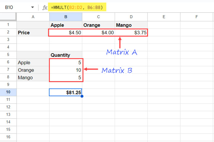
Assume Matrix 1 is in B2:D2 (prices of fruits), and Matrix 2 (quantities of fruits) is in B6:B8.
You can use the following MMULT formula to calculate the matrix product, which will be 81.25, representing the total price of the fruits:
=MMULT(B2:D2, B6:B8)Example 2: Matrix 1 with 3 Columns (1×3 Matrix) and Matrix 2 with 3 Rows (3×5 Matrix)
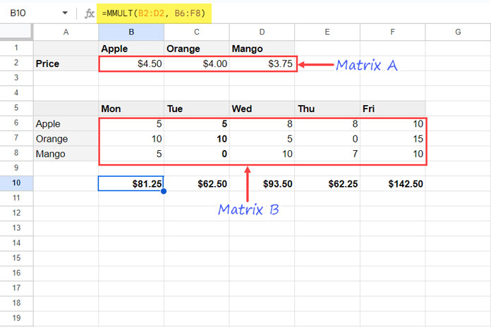
This time, Matrix 2 contains five columns representing sales quantities for each workday from Monday to Friday.
Matrix 1 (prices) is in the range B2:D2, and Matrix 2 (sales quantities) is in the range B6:F8.
The number of columns in Matrix 1 is 3, and the number of rows in Matrix 2 is also 3, satisfying the matrix multiplication rule.
To calculate the total sales amount for each workday, use the following MMULT formula:
=MMULT(B2:D2, B6:F8)Example 3: Matrix 1 with 3 Columns (2×3 Matrix) and Matrix 2 with 3 Rows (3×5 Matrix)

In this example, the prices are in two rows: B2:D2 contains the old prices, and B3:D3 contains the revised prices. Therefore, Matrix 1 is in the range B2:D3, making it a 2×3 matrix.
Matrix 2 is the same as in the previous example, with sales quantities in 5 columns in the range B6:F8.
The number of columns in Matrix 1 is 3, and the number of rows in Matrix 2 is also 3, satisfying the matrix multiplication rule.
To calculate the total sales amount for each workday based on old and revised prices separately, use the following MMULT formula:
=MMULT(B2:D3, B6:F8)I hope these examples clarify the practical use of the MMULT function in Google Sheets.
Common Errors
When using the MMULT function, you might encounter the #VALUE! error. If you do, hover your mouse pointer over the error to read the tooltip.
- If it says “MMULT has incompatible matrix sizes,” it means the matrices are not following the matrix multiplication rule.
- If it says “Function MMULT parameters expect number values,” make sure there are no empty cells or text in the range. If there are empty cells or text, and you need to keep them in the range, you can use the following workaround:
Wrap the matrices with the N function and enter the formula as an array formula.
Example:
=ArrayFormula(MMULT(N(B2:D3), N(B6:F8)))This will convert non-numeric values to 0s and resolve the issue.