


")


")

")
")
 in Excel & Google Sheets")


In the QUERY function, we use different types of values such as strings, numbers, dates, datetimes, times of day, and booleans for comparisons or assignments. These values are called literals. Each type of literal has a specific format in Google Sheets QUERY. This tutorial explains them with examples.
1. String Literals in Google Sheets QUERY
The correct way to use string literals in QUERY is to enclose them in string delimiters. You can use either single quotes (') or double quotes ("), but the latter is preferable. Here’s why.
Example Dataset:
The sample data consists of tradeshow (Expo) names, hosting country, city, and theme in columns A to D.
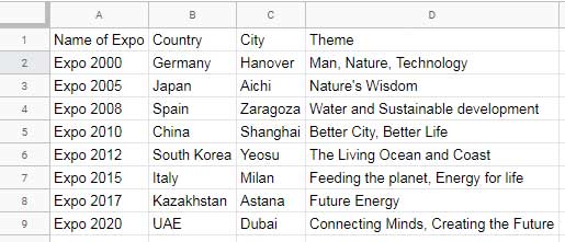
Filtering by City
To filter rows containing expos in Dubai, use the following formula:
=QUERY(A1:D, "Select * where C='Dubai' ", 1)In this formula, single quotes (') are used as string delimiters to enclose the text. However, you can also use double quotes:
=QUERY(A1:D, "Select * where C=""Dubai"" ", 1)Handling Apostrophes in Strings
If the string contains an apostrophe, the first formula will fail. For example, filtering “Nature’s Wisdom” in column D will cause an error. In such cases, use double quotes:
=QUERY(A1:D, "Select * where D=""Nature's Wisdom"" ", 1)Using Cell References for String Literals
If the search term (e.g., “Dubai”) is stored in cell F1, modify the formula as follows:
Using Single Quotes:
=QUERY(A1:D, "Select * where C='"&F1&"' ", 1)Using Double Quotes:
=QUERY(A1:D, "Select * where C="""&F1&""" ", 1)2. Number Literals in Google Sheets QUERY
Numbers are straightforward in QUERY since they can be specified directly in decimal notation.
Example Dataset:
Customers’ names (Column A) and outstanding receivables (Column B).
| Customer Name | Amount (USD) |
| A | $15,000.00 |
| B | $6,500.00 |
| C | $15,000.00 |
| D | $7,500.00 |
| E | $6,500.00 |
| F | $20,000.00 |
To filter customers with outstanding receivables greater than 10,000, use:
=QUERY(A1:B, "Select * where B >= 10000 ", 1)For dynamic filtering using a value from cell C1, use:
=QUERY(A1:B, "Select * where B >= "&C1&" ", 1)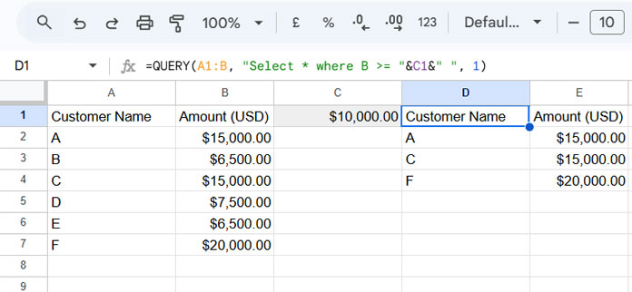
3. QUERY Literals: Date, DateTime, and Timeofday
Date, datetime, and time literals are similar to string literals but must be preceded by specific keywords and follow a defined format.
Date Literals
To filter employees whose contract end date is on or before 31/12/2025, use:
=QUERY(A1:B, "Select * where B <= date '2025-12-31' ", 1)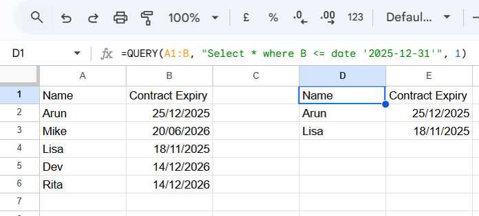
Format Rules:
- The date should be in
yyyy-mm-ddformat. - Enclose the date in single quotes (
'). - Precede the date with the date keyword.
Using a Cell Reference (C1 contains the date):
=QUERY(A1:B, "Select * where B <= date '"&TEXT(C1, "yyyy-mm-dd")&"' ", 1)The TEXT function ensures the correct format.
DateTime (Timestamp) Literals
To filter employees who checked in after 10:00 AM on 09/05/2019, use:
=QUERY(A1:B, "Select * where B >= timestamp '2019-05-09 10:00:00' ", 1)Format Rules:
- Use
yyyy-mm-dd hh:mm:ss[.sss]format. - Enclose the value in single quotes (
'). - Use the timestamp or datetime keyword.
Using a Cell Reference (F1 contains the datetime):
=QUERY(A1:B, "Select * where B >= datetime '"&TEXT(F1, "yyyy-mm-dd hh:mm:ss")&"' ", 1)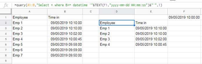
Timeofday Literals
If column B contains only time values, the QUERY formula would be:
=QUERY(A1:B, "Select * where B >= timeofday '10:00:00' ", 1)Format Rules:
- Use
hh:mm:ss[.sss]format. - Enclose the value in single quotes (
'). - Use the timeofday keyword.
Using a Cell Reference (F1 contains the time):
=QUERY(A1:B, "Select * where B >= timeofday '"&TEXT(F1, "hh:mm:ss")&"' ", 1)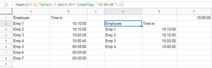
4. Boolean Literals in Google Sheets QUERY
Boolean literals can be TRUE or FALSE and used like number literals.
Column A contains names, and column B contains a TRUE/FALSE status.
To filter only TRUE values:
=QUERY(A1:B, "Select * where B = TRUE", 1)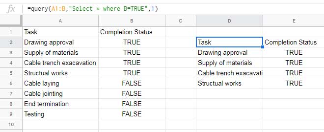
For dynamic filtering (if F1 contains TRUE or FALSE):
=QUERY(A1:B, "Select * where B = "&F1&" ", 1)Conclusion
I hope you find these formula examples useful for working with literals in Google Sheets QUERY. Understanding the correct syntax for string, number, date, datetime, timeofday, and boolean literals will help you write more efficient QUERY formulas. Enjoy!
Resources
- How to Use DateTime in a QUERY in Google Sheets
- How to Use Date Criteria in QUERY Function in Google Sheets
- How to Use Date Criteria in the FILTER Function in Google Sheets
- How to Hardcode DATETIME Criteria within FILTER Function in Google Sheets
- How to Extract Time from DateTime in Google Sheets: 3 Methods
- How to Use Cell References in Google Sheets QUERY
Hello, could you help me identify how to combine multiple criteria for 1 Col?
Say I need to import columns tagged as Started and Pending.
I have tried:
"where col 2 contains 'Started' and 'Pending'"and a bunch of others, but it doesn’t seem to work.Hi, J,
Here is an example.
=query({A1:D},"Select * where Col2 matches 'Started|Pending'",1)Hello,
I found that a value has brackets in mid of it [ex. 123(4)56 ], the below function doesn’t work correctly.
Could you please give me a hand to find out the error?
=QUERY(A27:G,"select * where not B matches '"&textjoin("|",true,'DATA'!C3:C)&"'")Hi, Jun,
Substitute
123(4)56with123\(4\)56Also, you may format the corresponding columns to text to avoid mixed-type data issues.