


")


")

")
")
 in Excel & Google Sheets")


Google Sheets makes it easy to calculate ISO week numbers with the ISOWEEKNUM function, but what if you need the actual dates instead of just the number? For example, given ISO week 12 of 2024, you may want to know that it starts on March 18 and ends on March 24. In this tutorial, I’ll show you how to return the week start (Monday) and end (Sunday) dates from a given ISO week number in Google Sheets with simple, reusable formulas.
Introduction
We can convert ISOWEEKNUM to date in Google Sheets using a similar approach to converting WEEKNUM to corresponding dates.
With the help of the WEEKDAY function, we can get a date (or a full date range) from a given week number.
I have already explained this for WEEKNUM here – Find the Date or Date Range from Week Number in Google Sheets.
Now let’s see the similar method to convert an ISOWEEKNUM to dates (week start and week end) in Google Sheets.
Before that, it’s important to understand the differences and similarities between WEEKNUM and ISOWEEKNUM.
For more details about both functions, you can also check my guide – The Complete Guide to All Date Functions.
WEEKNUM and ISOWEEKNUM: Differences and Similarities
Here are the key points to know before converting an ISO week number (ISOWEEKNUM) to dates in Google Sheets:
- Both functions take a date and return the corresponding week number.
- In WEEKNUM, you can specify a type argument (a number that defines which day the week starts on).
- There are ten types:
1, 2, 11, 12, 13, 14, 15, 16, 17, 21. For example, type1(or leaving it blank) means the week runs from Sunday to Saturday. - Type
21uses ISO8601 rules, where weeks run from Monday to Sunday.
The key difference:
- In ISO8601, the first week of the year is the one containing the first Thursday.
- This is exactly how ISOWEEKNUM works.
So, using WEEKNUM with type 21 is essentially the same as using ISOWEEKNUM.
Convert ISOWEEKNUM to Dates in Google Sheets
In our sample data, column B contains the customer names, column C holds the year, and column D lists the ISO week numbers representing the paying week. Using these details, we will calculate the pay start date (Monday) in column F and the pay end date (Sunday) in column G.
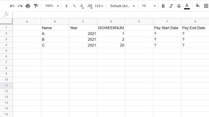
Find Pay Start and End Date from Paying Week Number (ISOWEEKNUM)
Let’s calculate the pay start (Monday) and pay end (Sunday) dates from ISOWEEKNUM in Google Sheets.
F2 formula (Start Date):
=LET(test, DATE(C2, 1, -2)-WEEKDAY(DATE(C2, 1, 3))+D2*7, IF(ISOWEEKNUM(test)=D2, test, ))G2 formula (End Date):
=LET(test, DATE(C2, 1, -2)-WEEKDAY(DATE(C2, 1, 3))+D2*7+6, IF(ISOWEEKNUM(test)=D2, test, ))Drag these formulas down.
Anatomy of the Formulas
This section breaks down the logic step by step so you understand how each part of the formula works before combining them into the final version.
Let’s start with a few key points:
- In ISO week numbering, the first Monday of Week 1 is always between December 29 and January 4.
- Example:
| If Thursday is | Then ISO Week 1 Starts (Monday) |
|---|---|
| Jan 1 | Dec 29 |
| Jan 2 | Dec 30 |
| Jan 3 | Dec 31 |
| Jan 4 | Jan 1 |
| Jan 5 | Jan 2 |
| Jan 6 | Jan 3 |
| Jan 7 | Jan 4 |
So, the first Monday immediately before January 5 will always be the start of ISO Week 1.
Finding the Monday of Any Date
To get the Monday of the week containing a given date:
=date - WEEKDAY(date) + 2To get the Monday strictly before the given date:
=date - WEEKDAY(date - 2)Here, we subtract 2 inside the WEEKDAY function. If we used date - 1, the formula would return Sunday (the day before Monday). Since we specifically want Monday, we go one step further and use date - 2.
As explained in the earlier table, ISO Week 1 always starts on the Monday that falls between December 29 and January 4, depending on which day the first Thursday of the year occurs.
So, to find that Monday in Google Sheets, we use the date immediately before January 5 of the given year:
=DATE(year, 1, 5)-WEEKDAY(DATE(year, 1, 3))This gives us the ISO Week 1 start date, which forms the base for converting ISOWEEKNUM to date in Google Sheets.
Final Formula for Week Start and End Dates
To get the anchor point, we first find the Monday of the last ISO week in the previous year:
=DATE(year, 1, -2)-WEEKDAY(DATE(year, 1, 3))DATE(year, 1, -2)→ gives December 29 of the previous year (as per the ISO table, ISO Week 1 can begin as early as Dec 29).WEEKDAY(DATE(year, 1, 3))→ finds the weekday of January 3 and helps adjust back to the last Monday of the previous year, which is also the start of the last ISO week of that year.
This Monday becomes the anchor date for calculating ISO weeks in the given year.
So the final formulas are:
Start date:
=DATE(C2, 1, -2)-WEEKDAY(DATE(C2, 1, 3))+D2*7Here, D2*7 shifts the anchor Monday forward by the correct number of weeks.
End date:
=DATE(C2, 1, -2)-WEEKDAY(DATE(C2, 1, 3))+D2*7+6The +6 moves from Monday to Sunday of the same ISO week.
The Role of LET and IF
The LET function assigns the formula result to the name test.
The IF condition checks whether the ISO week number of test matches the value in D2.
- If yes → it returns the start/end date.
- If not → it returns blank.
This prevents issues when the ISO week number entered is invalid.
Resources
- Calculate Week Number Within Month (1–5) in Google Sheets
- Find the Date or Date Range from Week Number in Google Sheets
- Weekday Name to Weekday Number in Google Sheets
- Reset Week Number in Google Sheets Using Formulas
- Convert Month Name to Month Number in Google Sheets
- Convert Month Numbers to Month Names in Google Sheets
This sadly fails for e.g.:
26/12/2022
27/12/2022
28/12/2022
29/12/2022
30/12/2022
by incorrectly setting the isoweek’s start date to 01/01/2022
Hi, Mateusz J,
Thanks for letting me know, and sorry for the unforeseen error.
I’ll update my formulas ASAP. Please check back later.