Managing schedules, subscriptions, or recurring tasks in Google Sheets can get tricky when dates repeat across rows. Imagine you have a list of items that are subscribed every month — you might duplicate the same row 12 times for a year. Without adjusting the dates, all 12 rows would show the same start date, which makes tracking and reporting confusing.

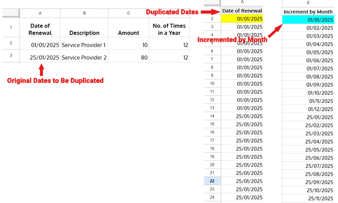
This is where automatically adjusting duplicate dates in Google Sheets becomes a lifesaver. In this tutorial, we’ll walk you through how to:

• Duplicate rows for recurring events or subscriptions.
• Increment dates by day, month, or custom intervals.
• Handle open ranges and avoid errors with blank rows.

By the end, you’ll have a clean, automated workflow that saves time and reduces mistakes when dealing with repeating dates.

Sample Data for Duplicate Records

Here’s the sample data we’ll use in Sheet1 (A1:D):

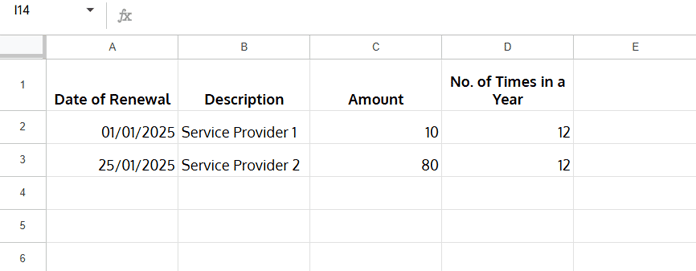
We want to duplicate each row based on the “No. of Times in a Year” column.

Duplicate Records Formula

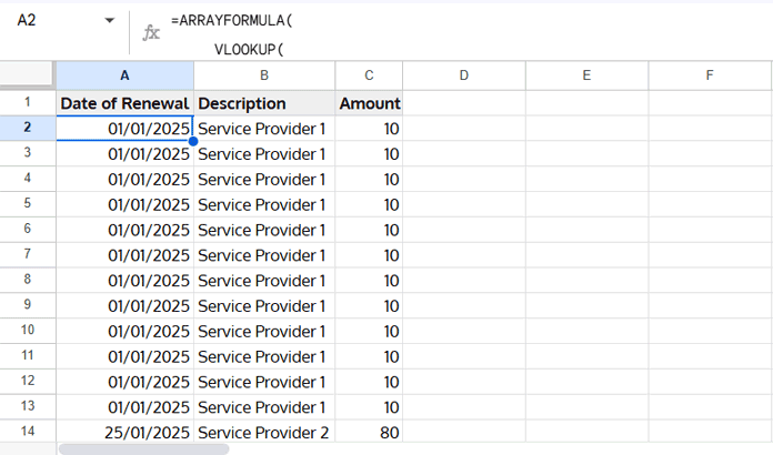
To duplicate the records automatically in Sheet2, use the following formula in cell A2:

=ARRAYFORMULA(
     VLOOKUP(
        TRANSPOSE(SPLIT(QUERY(REPT(ROW(Sheet1!A2:A)&" ", Sheet1!D2:D),,9^9), " ")),
        {ROW(Sheet1!A2:A), Sheet1!A2:D},
        {1, 2, 3}+1,
        0
     )
)

Notes:

• Sheet1!A2:A → first column of your data.
• Sheet1!D2:D → number of times to repeat each record.
• Sheet1!A2:D → actual data range.
• {1, 2, 3} → columns to repeat.

After this, select column A, then go to Format > Number > Date to ensure proper date formatting.

For a deeper dive on duplicating rows, you can check out How to Insert Duplicate Rows in Google Sheets.

Automatically Adjust Duplicate Dates by Month

Once rows are duplicated, the next step is to increment the dates so each duplicate shows the next month.

Our sample data includes a category column (like “Description”), which is important because if multiple categories share the same date, we want to increment dates per category, not across the entire column.

Formula for Simple Increment (No Categories)

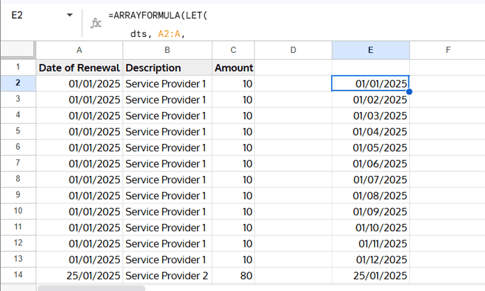
If you just want to increment dates without considering categories, use this formula in a new column:

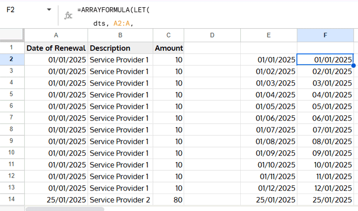
=ARRAYFORMULA(LET(
    dts, A2:A,
    rc, COUNTIFS(dts, dts, SEQUENCE(ROWS(dts)), "<="&SEQUENCE(ROWS(dts)))-1,
    IFERROR(EDATE(dts, rc))
))

Explanation:

• EDATE(start_date, [months]) → advances each date by the number of months specified in [months].
• rc → a running count of duplicates starting at 0, representing the number of months to add. For example, if a row is duplicated 12 times, rc will count 0, 1, 2…11, effectively adding 0 to 11 months to the original date.
• ARRAYFORMULA → allows the formula to apply automatically to the entire column.

Format the results as Date to see the incremented monthly schedule.

Formula for Increment by Category

If your dataset has a category column, like “Description”, you need to tweak the formula so that duplicates are counted per category. Without this, duplicates from other categories with the same date would incorrectly affect the count.

=ARRAYFORMULA(LET(
    dts, A2:A,
    cat, B2:B,
    rc, COUNTIFS(dts&cat, dts&cat, SEQUENCE(ROWS(dts)), "<="&SEQUENCE(ROWS(dts)))-1,
    IF(dts, IFERROR(EDATE(dts, rc)),)
))

Note:

You won’t see any differences between the category and non-category formulas in this example because there are no duplicate subscription periods in the sample data. The distinction only matters when multiple rows share the same start date within different categories.

How it works:

1. dts → stores the date column.
2. cat → stores the category column.
3. COUNTIFS(dts&cat, dts&cat, SEQUENCE(ROWS(dts)), "<="&SEQUENCE(ROWS(dts)))-1 → calculates a running count for each date within each category.
4. EDATE(dts, rc) → adds the running count as months to each original date.
5. IF(dts, ..., ) → ensures empty rows are ignored.

This ensures that:

• Multiple categories with the same start date are handled separately.
• Dates increment correctly within each category.
• Blank rows do not produce errors.

Why This Formula Works

Even though it looks complex, it’s essentially combining three things:

1. EDATE → advances dates by a specific number of months.
2. COUNTIFS + SEQUENCE → creates a running count of duplicates (per category if needed).
3. LET → organizes variables (dts, cat, rc) to make the formula easier to read and maintain.

For a deeper understanding of running counts, see Running Count in Google Sheets: Formula Examples.

Automatically Adjust Duplicate Dates by Day

If you need to increment by days instead of months, the formula is simpler:

=ARRAYFORMULA(LET(
    dts, A2:A,
    rc, COUNTIFS(dts, dts, SEQUENCE(ROWS(dts)), "<="&SEQUENCE(ROWS(dts)))-1,
    IF(dts, dts+rc,)
))

And with categories:

=ARRAYFORMULA(LET(
    dts, A2:A,
    cat, B2:B,
    rc, COUNTIFS(dts&cat, dts&cat, SEQUENCE(ROWS(dts)), "<="&SEQUENCE(ROWS(dts)))-1,
    IF(dts, dts+rc,)
))

This increments each duplicate date by one day for each repetition, automatically handling multiple categories.

Wrapping Up

Using this method, you can:

• Automatically duplicate rows based on a frequency column.
• Increment duplicate dates by month or day.
• Handle multiple categories without errors.
• Create a scalable, automated workflow in Google Sheets for subscriptions, schedules, or recurring events.

No more manually updating 12 rows for each subscription — let Google Sheets do the work for you.

Resources

• Find Missing Sequential Dates in a List in Google Sheets
• How to Fill Missing Dates in Google Sheets (Categorized & General)
• Expand Dates and Assign Values in Google Sheets (Array Formula)