


")


")

")
")
 in Excel & Google Sheets")


The NPV Function in Google Sheets is categorized under the financial functions (Insert > Function > Financial).
The purpose of the NPV function is to calculate the net present value (NPV) of an investment. For the calculation, the function requires two main inputs: the discount rate and a series of periodic (future) cash flows.
As you may already know, money earned today is more valuable than money earned in the future because the money you have now can earn interest. The discount rate (interest rate) in the NPV calculation addresses this time value of money.
We need to use the NPV function in Google Sheets in a specific way to get the correct net present value of future cash flows.
The reason is that the NPV function is similar to the PV function. The key difference is that the NPV function allows for variable-value cash flows, whereas the PV function assumes constant-amount periodic payments. I’ll explain this with an example later in this tutorial.
Let’s dive into how to use the NPV function in Google Sheets the right way.
Syntax and Arguments of the NPV Function in Google Sheets
Syntax:
NPV(discount, cashflow1, [cashflow2, ...])Arguments:
- discount: The rate of discount for the investment over the length of one period.
- cashflow1: The first (future) cash flow.
- cashflow2, …: Additional (future) cash flows.
Points to Note:
- cashflow1, cashflow2, … must be equally spaced in time and occur at the end of each period.
- A cashflow should be positive (+) if it represents income, or negative (−) if it represents payments, from the investor’s perspective.
- The NPV function in Google Sheets uses the order of the cash flows to interpret their sequence. Ensure you enter the payment and income values in the correct order.
Examples of Net Present Value Calculation in Google Sheets
The NPV function is actually one of the easiest financial functions to learn in Google Sheets.
For example, let’s consider an investment in an upcoming project. Using the NPV function in Google Sheets, we can make an informed decision about whether it’s worth investing in the project.
Here’s a basic example to demonstrate how to use the NPV function.
Example 1 – Investment Decision
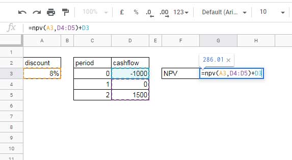
Assume the project requires an initial investment of $1,000, and we expect $0 income in the first period (first year) and $1,500 in the second period (second year).
If the annual discount rate is 8%, the NPV would be 286.01.
NPV function usage in Google Sheets:
=NPV(A3, D4:D5)Result: 1,286.01
To calculate the net present value (NPV), we must subtract (or add, due to the negative value) the initial investment value from the present value (PV).
=NPV(A3, D4:D5) + D3Result: 286.01
We can also use an IF statement to return a “YES” or “NO” answer to help decide whether to invest in the project.
=IF(NPV(A3, D4:D5) + D3 > 0, "YES", "NO")Example 2 – NPV vs. PV (Fact Check)
To further understand the NPV function, let’s compare it to the PV function by using fixed-value cash flows instead of variable-value ones.
Input Values for NPV:
- Discount: 8%
- There are 5 future cash flows, each amounting to $1,500.
| A | B | C |
| discount | period | cash flow |
| 8% | 0 | -4500 |
| 1 | 1500 | |
| 2 | 1500 | |
| 3 | 1500 | |
| 4 | 1500 | |
| 5 | 1500 |
The following NPV formula would return 5,989.07 as the net present value:
=NPV(A2, C3:C7)Note: This value represents the present value (PV) since we haven’t considered the initial investment value in cell C2, which is -4,500.
Let’s now use these elements in the PV function:
| A | B |
| rate | 8% |
| number_of_periods | 5 |
| payment_amount | 1500 |
The following PV formula would return -5,989.07, and that tells us everything!
=PV(B1, B2, B3)That’s all about how to use the NPV function in Google Sheets. Thanks for reading, and enjoy exploring Google Sheets’ financial functions!