This article is a child post of the hub Date Logic in QUERY Function in Google Sheets. It explains how to use the MONTH function in Google Sheets QUERY, including how it differs from the worksheet MONTH function and how to use it for month-wise summaries.
What Is the MONTH Function in Google Sheets QUERY?
The MONTH function is a scalar function in Google Sheets QUERY. It returns a month number from a date or DateTime (timestamp) column.
Key characteristics
- It is a scalar function, so it returns one value per row (unlike aggregate functions, which return one value per group).
- When you wrap a column with
MONTH(), QUERY changes the column label automatically.- For example, if column C is labeled Purchase Date, the output label becomes:
month(Purchase Date)
- For example, if column C is labeled Purchase Date, the output label becomes:
Basic syntax example
=QUERY(C1:C, "select month(C)", 1)MONTH Function in QUERY vs Worksheet MONTH Function
Although both functions extract month numbers, they behave differently.
Important difference
- QUERY MONTH function → returns zero-based month numbers
- January = 0
- February = 1
- …
- December = 11
- Worksheet MONTH() function → returns 1–12
- January = 1
- February = 2
- …
- December = 12
You May Like: Google Sheets: The Complete Guide to All Date Functions
This difference often surprises users and is a common source of errors.
Later in this tutorial, you’ll learn how to convert zero-based months into normal month numbers.
This tutorial is part of the Date Logic in QUERY hub, which covers date criteria, month-based filtering, and DateTime handling in Google Sheets QUERY.
Purpose of the MONTH Function in Google Sheets QUERY
The MONTH function in QUERY is mainly used for two purposes:
- Return month numbers from a date or DateTime column
- Group and summarize data by month
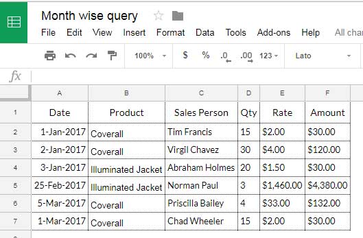
Sample Data Structure
Assume the following columns:
- Column A – Date
- Column B – Product
- Column C – Salesperson
- Column D – Quantity
- Column E – Rate
- Column F – Amount

Return Month Numbers from a Date Column
To extract month numbers from the dates in column A, use:
=QUERY(A1:A, "select month(A)",1)Insert this formula in the top row of any empty column.
month(Date)
0
0
0
1
2
2
Note: The returned month numbers are zero-based.
Group Data by Month Using QUERY
Now let’s see how to summarize data month-wise using the MONTH function.
Goal
Create a report that shows the total sales amount per product for each month.
For this example, we’ll use only three columns:
- Column A – Date
- Column B – Product
- Column F – Amount
Example: Month-Wise Summary Using MONTH Function
=QUERY(A1:F,
 "select month(A), B, sum(F)
  where A is not null
  group by month(A), B",
  1)
What this formula does
month(A)converts dates into zero-based month numbersgroup by month(A), Bgroups the data by month and productsum(F)aggregates the Amount column
| month(Date) | Product | sum Amount |
|---|---|---|
| 0 | Coverall | 150 |
| 0 | Illuminated Jacket | 30 |
| 1 | Illuminated Jacket | 4380 |
| 2 | Coverall | 162 |
The result shows:
- Month number (0–11)
- Product name
- Total amount for each product in each month
Related: What Is the Correct Clause Order in Google Sheets QUERY?
How to Convert Zero-Based Month Numbers
Since QUERY returns months as 0–11, you may want standard month numbers (1–12).
You can do this by adding +1 to the MONTH function.
=QUERY(A1:F,
 "select month(A)+1, B, sum(F)
  where A is not null
  group by month(A)+1, B",
  1)
Why this works
- QUERY counts months starting from 0
- Adding
+1converts them to the usual month numbering
This produces a cleaner and more familiar month-wise summary.
| sum(month(Date)1()) | Product | sum Amount |
|---|---|---|
| 1 | Coverall | 150 |
| 1 | Illuminated Jacket | 30 |
| 2 | Illuminated Jacket | 4380 |
| 3 | Coverall | 162 |
Key Takeaways
- The
MONTHfunction in Google Sheets QUERY is a scalar function. - It returns zero-based month numbers (0–11).
- It is commonly used for month-wise grouping and summarization.
- Add
+1to convert zero-based months into standard month numbers.
That’s how to use the MONTH function in Google Sheets QUERY to extract and summarize data by month.
Thanks for reading, and enjoy exploring date logic in QUERY!


I used the Month function and it gives values from 0 to 11. January dates give Month as zero etc. Why?
Hi, Arvind Pradhan,
I’ve already explained the same within this tutorial.
It’s numbered 0-11. To get 1-12, you should add 1 to the returned month numbers.
Eg.
Use
Month(A)+1instead ofMonth(A).