The Month function, one of the scalar functions in Google Sheets Query, returns the month numbers from a date or timestamp column.
Here are two salient features of the Month function in Query.
- It’s a scalar function, so it returns one value per row, unlike the aggregate functions, which return one value per group.
- It changes column names when wrapping it with columns. If the field label of column C is “Purchase Date,” the following formula will replace it with “month(Purchase Date).”
=query(C:C,"Select month(C)")How does it differ from its counterpart worksheet function?
When we compare the Month scalar function in Google Sheets Query with the Month() worksheet function, which is part of Date Functions, the former returns a slightly different result.
Here, the month numbers are zero-based. As a result, the month number of January will be 0, February will be 1, and so on.
You can change this behavior with a simple trick which I’ll explain later.
Purpose of the Month Function in Google Sheets Query
Here are the two purposes of the Month scalar function in Google Sheets Query.
- Return month numbers from columns.
- Group a date or DateTime (timestamp) column by months.
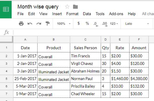
Sample Data:

Return Month Numbers:
Insert =query(A:A,"Select month(A)") in the top row of any blank column to extract month numbers from the dates in column A.
Group by Month Numbers:
Now let’s learn in detail how to convert and summarise data based on the month numbers.
We can use the above data and summarize “Product” month-wise.
The purpose is to get the total sales amount of each product in different months.
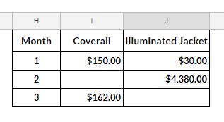
Here is our expected result.

There are two steps involved in generating the above summary.
You can learn that below and get a clear picture of using the Month function in Google Sheets Query.
Using the Month Function in Google Sheets Query to Summarize Data
We are using only three columns in the above sample data: A (Date), B (Product), and F (Amount).
There are two steps: Group & Summarize and Pivot & Label Format.
With these, we can learn how to use the Month function in Google Sheets Query to convert dates to months and group by month numbers (not month text).
1. Grouping and Summarizing
There are two columns in the SELECT clause of the below Query formula: Month(A) and B, and the first one converts dates to zero-based month numbers.
=query(A1:F,"Select Month(A),B, Sum(F) where A is not null group by Month(A),B",1)The formula groups these selected columns using the GROUP BY keyword combination (clause) and then aggregates (sum) column F.
Related: What is the Correct Clause Order in Google Sheets Query?
How to Convert Zero-Based Month in Query?
=query(A1:F,"Select Month(A)+1,B, Sum(F) where A is not null group by Month(A)+1,B",1)I used the Month function in the above Query as Month(A)+1 in both the SELECT and GROUP BY clauses.
It is simply because, in Query, the months are counted/numbered from 0 to 11 (zero-based).
So, the Month function would return 0 for January, 1 for February, etc.
By adding 1 to the returned value, we can get the usual month number for our purpose.
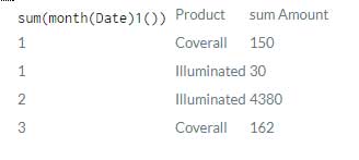
Please see the result of the above formula.

It is not our expected result! We should pivot this output and format the labels for that.
Find those steps below.
2. Pivot Grouped Data and Formatting Labels
To pivot the data by “Products,” remove the relevant column B from the grouping.
Then use it with the PIVOT clause.
=query(A1:F,"Select Month(A)+1, Sum(F) where A is not null group by Month(A)+1 pivot B",1)Finally, use the LABEL clause to rename sum(month(Date)1()) (please see the above image), the column name “Date” replaced by the Month scalar function, with “Month.”
=query(A1:F,"Select Month(A)+1, Sum(F) where A is not null group by Month(A)+1 pivot B label Month(A)+1'Month'",1)Scroll up and see the above Screenshot # 2 for the output.
This way, we can use the Month function in Google Sheets Query and make a month-wise summary report.


I used the Month function and it gives values from 0 to 11. January dates give Month as zero etc. Why?
Hi, Arvind Pradhan,
I’ve already explained the same within this tutorial.
It’s numbered 0-11. To get 1-12, you should add 1 to the returned month numbers.
Eg.
Use
Month(A)+1instead ofMonth(A).