The Delta function in Google Sheets is categorized under the Engineering function. This post includes the purpose, syntax, and formula (array/non-array) examples of this simple to use function in Docs Sheets.

Personally, if I want to test whether values in any two columns are equal in row-wise, I would prefer to use this function. But there are equivalents that you can find at the end of this post.

Let’s begin with the purpose of the Delta function in Google Sheets.

Purpose:

The purpose of the Delta function is pretty simple to understand. It compares two numeric values and returns 1 if they match, else 0.

Syntax:

DELTA(number1, [number2])

There are two arguments, for two numbers to test/compare for equality, in this function in Google Sheets.

If you omit the second argument (which is an optional argument) the function will compare the first number with 0 for equality.

With the help of this function, you can also compare two dates, two timestamps and also time entries.

As a side note, to compare strings or other values including date, number, time, timestamp, etc., you can use the EQ function in Google Sheets. Please do note that instead of 1 or 0, EQ returns TRUE or FALSE.

To learn EQ function and other comparison operators in Sheets please check the following guide – Comparison Operators in Google Sheets and Equivalent Functions.

Formula Examples to the Delta Function in Google Sheets

Here are a few Delta formula examples.

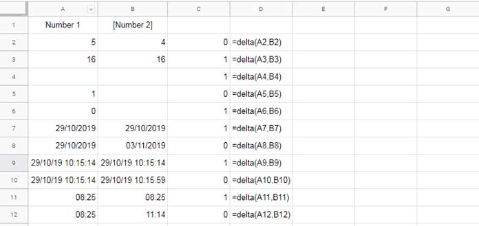
Compare Two Numbers and Return 1 if Match, Else Return 0:

=delta(100,100)

Result: 1

=delta(22,25)

Result: 0

Compare Two Dates and Return 1 if Match, Else Return 0:

=delta(date(2019,10,29),today())

The above formula compares the date 29/10/2019 with today’s date and will return 1 if both the dates are the same, else 0.

Please note that the Delta function treats a blank cell as the same as a zero.

Delta in Array Use

Here is one real-life example of the use of the Delta function in Google Sheets.

I have quotations from two vendors for 10 different products as below.

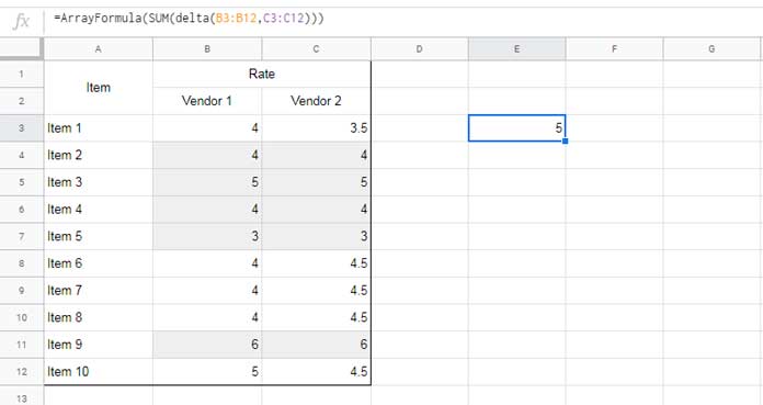
Using the SUM function with Delta, we can count the number of items the vendors match their prices.

The formula for the same, which you can find in cell E3, is as below.

=ArrayFormula(SUM(delta(B3:B12,C3:C12)))

You can also use different formulas to get the above count. Here are two such formulas that immediately came to my mind.

Formula 1:

=ArrayFormula(sum(--eq(B3:B12,C3:C12)))

Formula 2:

=ArrayFormula(SUM(--(B3:B12=C3:C12)))

Similarly, you can compare dates in two columns like whether the ordered date and despatched date are the same.