 in Google Sheets")

")

")


")


")


To sort pie slices in a pie chart, you need to sort the data points in ascending or descending order. However, this won’t work when you use the Aggregate feature within the chart settings. In that case, you should create a helper range using QUERY or Pivot Table and use that range for the chart. We’ll see all these options in this tutorial on how to sort pie slices in Google Sheets.
Purpose of a Pie Chart
A pie chart is used to show how a whole is divided into parts.
For example, out of 100%, what percentage of website traffic is contributed by search engines, AI tools, social media platforms, and direct traffic?
It visually represents data as slices of a circle, with each slice corresponding to a category’s proportion of the total. In the example above, there would be four slices once you create the chart with the data.
Pie charts simplify comparisons and make it easy to see differences at a glance.
Why Should You Sort Pie Slices?
Sorting pie slices can actually make a big difference, depending on your goal. Here are a few reasons why you might want to sort the slices:
- Better readability: Sorted pie slices — whether ascending or descending — offer better clarity.
- Highlight key categories: Sorting allows the most significant categories to stand out immediately, which is useful if you want to draw attention to the biggest contributors.
- Cleaner and more professional look: A sorted pie chart looks more polished and intentional, rather than random or messy.
- Save time: It saves time when checking percentages, especially when slices are almost similar in size but slightly different.
Now, let’s move to the actual steps on how to sort pie slices in Google Sheets.
Sorting Pie Slices When No Aggregation Is Needed
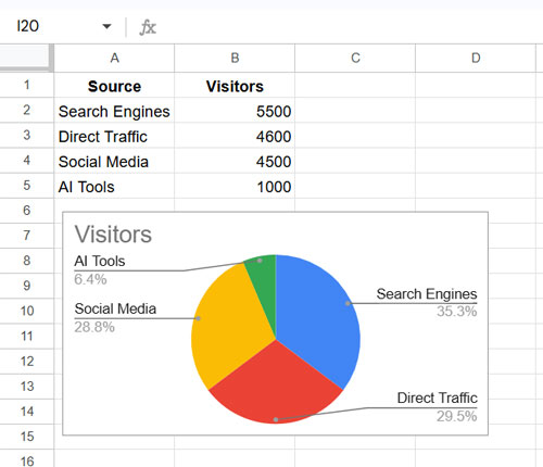
Imagine you have a website and you get visitors as follows:
| Source | Visitors |
| Search Engines | 5500 |
| AI Tools | 1000 |
| Social Media | 4500 |
| Direct Traffic | 4600 |
If the data is in A1:B5, you can create a pie chart with sorted slices by following these steps:
Step 1: Sorting the Data
- Select
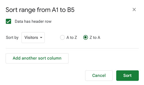
A1:B5. - Click Data > Sort Range > Advanced range sorting options to open the sort window.
- If your range contains a header row, select “Data has header row.”
- Sort by: “Visitors” (or Column B if you don’t have a header row).
- Check Z → A to sort the site traffic column from largest to smallest. (We usually sort pie slices in descending order so that, clockwise, slices appear from largest to smallest.)
- If you want the slices to appear in the opposite (anticlockwise) order, sort A → Z instead.
- Click Sort.
Step 2: Creating the Pie Chart with Sorted Slices
- Select
A2:B5. - Click Insert > Chart.
- Under the Setup tab, select Pie Chart.
This will create a pie chart with sorted slices in Google Sheets!
Sorting Pie Slices When Aggregation Is Needed
Sometimes you may have multiple occurrences of the same category. For example, consider your expense sheet:
| Expense | Amount |
| Rent | 1500 |
| Groceries | 800 |
| Groceries | 1000 |
| Transportation | 25 |
| Utilities | 100 |
| Transportation | 500 |
| Transportation | 100 |
| Entertainment | 100 |
When you want to create a pie chart and sort slices for this type of data, you should follow this approach:
Step 1: Aggregating the Data
Assuming your data is in A1:B with or without a header row, in cell D1, enter the following QUERY formula:
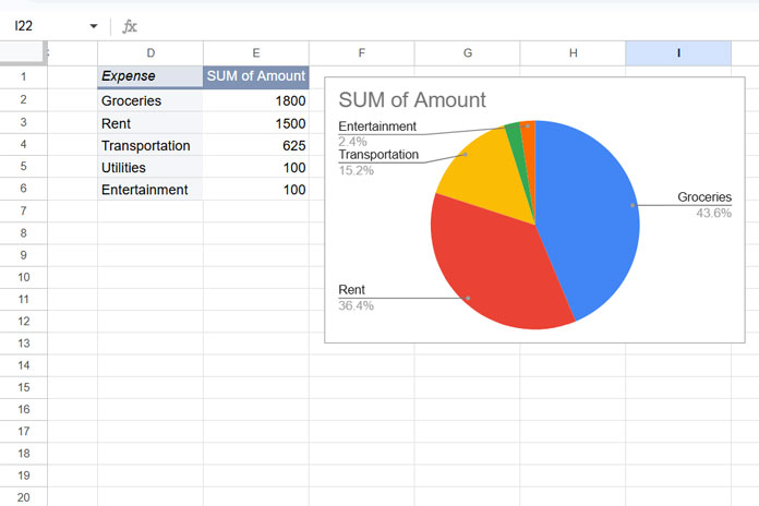
=QUERY(A1:B, "Select Col1, Sum(Col2) Where Col1 is Not Null Group By Col1 Order By Sum(Col2) Desc")It will return the following output (the header labels will be different if your source data does not have headers):
| Expense | sum Amount |
| Groceries | 1800 |
| Rent | 1500 |
| Transportation | 625 |
| Entertainment | 100 |
| Utilities | 100 |
Additional Tip:
You can alternatively use the following approach to prepare the sorted data for your pie chart:
- Select A1:B
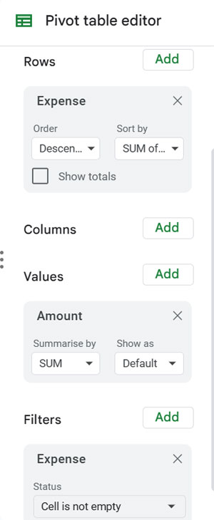
- Click Insert > Pivot table
- Choose Existing sheet
- In the field below, enter D1
- Click Create
- In the sidebar panel, add Expense under Rows and Amount under Values
- Under Rows, uncheck Show totals, set the order to Descending, and select Sort by Sum of Amount
- Add Expense under Filters, choose Filter by condition > Cell is not empty, and click OK
This also helps you organize the data properly for how to sort pie slices in Google Sheets.
Step 2: Creating the Pie Chart with Sorted Slices
- Select the output in
D2:E. - Insert a pie chart as earlier.
Now you’ll have a pie chart with sorted slices, even when the original data had multiple occurrences!
That’s all about how to sort pie slices in Google Sheets — whether or not aggregation is needed!