Show Vertical Gridlines in Google Sheets Charts (Horizontal Axis Fix)

If you’ve ever tried to add horizontal axis gridlines in Google Sheets (i.e., vertical lines across the chart) and couldn’t find the option in the chart editor — you’re not alone.
(These are technically gridlines aligned to the horizontal axis, which appear vertically across the chart — often called vertical gridlines.)

Sometimes, even if you do manage to enable them, you might notice missing or irregular X-axis labels. In this post, we’ll tackle both issues and walk through a few easy solutions.

Table of Contents

Why Horizontal Axis Gridlines Are Missing in Your Google Sheets Chart

Google Sheets does let you customize horizontal and vertical axis gridlines from the Chart Editor. But if you’re not seeing vertical gridlines (which align with the horizontal axis), here’s the likely reason:

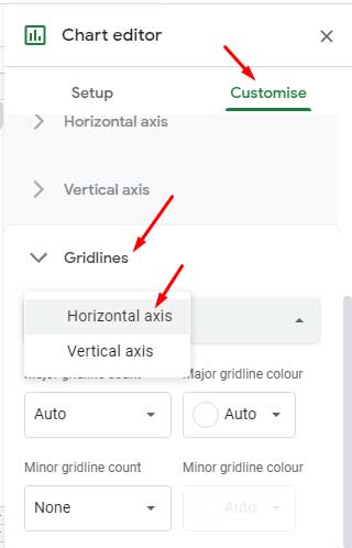
You need to set the gridline count under:
Chart Editor > Customize > Gridlines and Ticks > Horizontal Axis > Major Gridline Count
Change it from “None” to “Auto” or any number between 1 and 10.

Still not seeing that option? Here are a few common reasons:

Your X-axis values are text, not numbers or dates. Gridlines can’t align to string values.
“Treat Labels as Text” is enabled in the chart editor. That disables the gridline control.
You’ve enabled “Aggregate” in the chart setup, which can block gridline options.

Let’s break that down with an example.

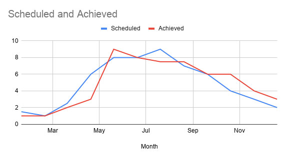
Sample Data #1 (Gridlines Missing)

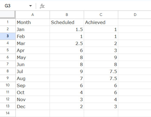
Sample data with month names used as text labels on the X-axis

If you use this data in a Line Chart, the month values (text) on the X-axis prevent the horizontal axis gridlines from appearing.

What to Do Instead

Change the month values to actual dates:

In A2, enter 01/01/2024 (or any start date), and in A3, enter 01/02/2024.
Then select both cells and drag the fill handle down to fill the rest of the column.
(Note: These dates are in DD/MM/YYYY format — adjust based on your sheet’s locale.)

Now format the column to display only the month abbreviation:
Go to Format > Number > Custom Number Format and type mmm.

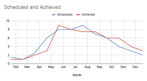
Now, Google Sheets recognizes the X-axis as dates — which allows the vertical gridlines to appear.

How to Display Vertical and Horizontal Gridlines in Google Sheets

Once your X-axis uses actual dates or numbers, here’s how to plot the chart with both sets of gridlines:

Steps to Insert a Line Chart with Gridlines

Select the data range A1:C13.
Click Insert > Chart.

Under the Setup tab:

Chart type: Line chart
Aggregate: Off
Switch rows/columns: Off
Use row 1 as headers: On
Use column A as labels: On
Uncheck “Treat labels as text”

You should now see both vertical and horizontal gridlines on your chart.

Line chart showing vertical and horizontal gridlines with partial X-axis labels

What If X-Axis Labels Go Missing?

With gridlines enabled, you might notice some months are missing from the X-axis. Here’s why:

Google Sheets tries to space out date labels to avoid clutter.
But you can bring back all the labels by adjusting the gridline count.

Go to:
Customize > Gridlines and Ticks > Horizontal Axis
Under Major Spacing Type, select Count.
Then set Major Count to 10.

Chart editor's Customize tab displaying horizontal axis gridline settings

This forces Sheets to show all X-axis labels while keeping vertical gridlines.

Line chart with complete X-axis labels and gridlines fully visible

Keep Gridlines When Aggregating Chart Data

If you enable Aggregate in the chart setup, you lose control over horizontal axis gridlines.

Instead, try this:

Use a QUERY Formula to Summarize Your Data

Sample Data #2 (Sheet1!A:C):

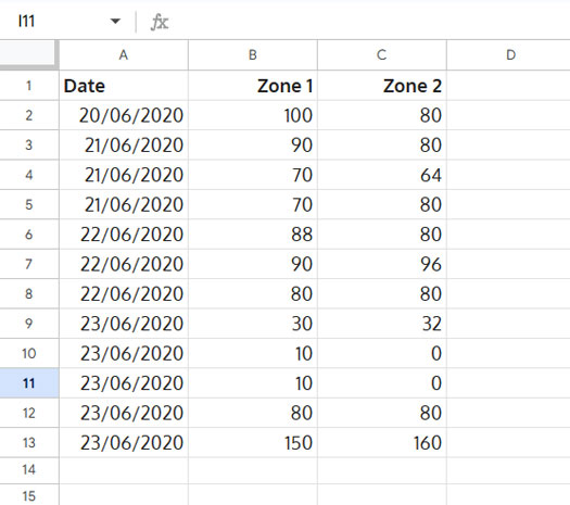
Raw date-based dataset prepared for aggregation using QUERY or pivot table.

Now use this in Sheet2!A1:

=QUERY(
  Sheet1!A:C,
  "select A, sum(B), sum(C) where A is not null group by A label A 'Date', sum(B) 'Zone 1', sum(C) 'Zone 2'",
  0
)

Or use a Pivot Table:

Select A1:C
Go to Data > Pivot Table > New Sheet
Set Date as Rows, Zone 1 and Zone 2 as Values (Summed)
Under Filters, uncheck (Blanks) if needed

Create your chart from this summary, and you’ll retain horizontal axis gridlines — as long as the X-axis is treated as numeric (not text).

Conclusion

To enable horizontal axis gridlines (vertical lines) in Google Sheets charts:

Make sure your X-axis values are numeric (dates, numbers, etc.).
Avoid enabling “Treat Labels as Text” unless you want labels over gridlines.
Don’t use Aggregate — instead, pre-summarize your data using QUERY or a Pivot Table.

This small setup tweak makes your charts easier to read and far more professional-looking.

Enjoy!