How to Properly Concatenate Start Time with End Time in Google Sheets

Recently I’ve helped one of my readers to concatenate a start time with an end time in his ‘preferred’ way in Google Sheets.

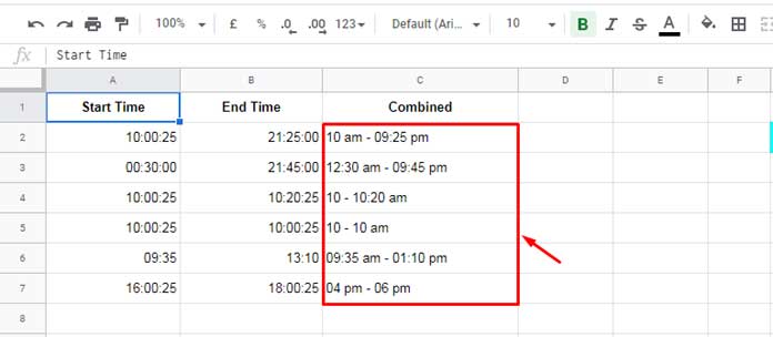
The preferred way was combining a 24 hr start and end time and then formatting it to a 12 hr start and end time, that also keeping the am/pm in the output.

Such concatenating of time values also involves removing some unwanted substrings/characters from the output (‘am’ repetition) which I will explain later.

So in this new Google Sheets tutorial, I am going to explain how to properly concatenate a start time with an end time in Google Sheets.

The start and end times are in two columns. I want to combine it into a single column output keeping the required (preferred) time format.

The process involves 5 helper columns. But in the final formula, we can remove all the helper columns by combining the formulas into one. Let’s begin.

Combining Two Time Cells in Google Sheets and Formatting Issue

Here is an important time formatting tip associated with concatenating time cells.

Normally when we concatenate a start time with an end time using the ampersand, the output may lack the time formatting.

Please see the below example.

Start Time	End Time
10:00:25	21:25:00

If we concatenate the above start time in cell A2 with the end time in cell B2 in Google Sheets, the formula and the result would be as follows.

=A2&" "&B2

Result: 0.416956018518519 0.892361111111111

Frustrating, right?

The output will be different if we concatenate a start time with an end time using either of the functions JOIN or TEXTJOIN.

=join(" - ",A2:B2)
=textjoin(" - ",true,A2:B2)

Result: 10:00:25 – 21:25:00

This result is OK to some extent now. But what I want is something different as below.

Expected Result: 10 am – 09:25 pm

I don’t want to display the seconds and remove minutes if it’s 00. Also, I want to include the am/pm which represents the periods in a 12-hour clock.

In addition to this, I just don’t want to repeat the ‘am’ if the start time and end time fall in the first half of the day (first period of 12-hour clock). Didn’t get?

Please see the 4th and 5th row in the example below.

Example - Concatenate Start Time with End Time in Google Sheets

Concatenating 12 Hr or 24 Hr Start Time with 12 Hr or 24 Hr End Time in the Normal Way

We can make use of the TEXT function to combine a 12 hr or 24 hr start time with a 12 hr or 24 hr end time in Google Sheets.

See how I am going to use the TEXT function with the JOIN function as well as with the & to concatenate a start time with an end time in Google Sheets.

Time Formatting and Combining Using TEXT and Ampersand:

=text(A2,"hh:mm am/pm")&" - "&text(B2,"hh:mm am/pm")

Time Formatting and Combining Using TEXT and JOIN:

=join(" - ",text(A2,"hh:mm am/pm"),text(B2,"hh:mm am/pm"))

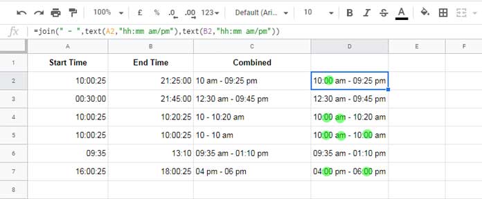
I am applying the last formula in cell D2 and then dragging it down to copy the formula down.

Combining Two Time Cells in Normal Way - Google Sheets

Alternatively, we can use an array formula in cell D2 and let it automatically expand to the range D2:D7. In this case, we can use the Text and Ampersand combo only.

=ArrayFormula(text(A2:A7,"hh:mm am/pm")&" - "&text(B2:B7,"hh:mm am/pm"))

Yes! The ampersand based concatenating of start time with end time has the array formula advantage over the TEXT and JOIN combo!

See how the output in column D is different from the expected output in column C. I think the combined start and end times in column C are more reader-friendly.

Are you interested to ‘properly’ concatenate a start time column with an end time column in Google Sheets as above in column C? Then read on to get the formula, that also, step-by-step.

Removing Extra Strings After Combining Start Time with End Time in Google Sheets

First, we will properly concatenate the start time in cell A2 with the end time in cell B2. Later we can apply the formula to the entire column A and B.

There are four steps involved. In these four steps, there are a total of 5 formulas required to combine the start and end time in a customized way in Google Sheets.

Steps to Concatenate Start and End Time in Google Sheets

1. Remove Minutes from Time if Minutes are Zero

The following TEXT formula in Google Sheets conditionally formats the time in cell A2 to 12-hour format.

=text(A2,if(minute(A2)=0,"HH am/pm","HH:MM am/pm"))

The formula removes the minutes if 00 else retains the minutes. The IF function does that. Then the TEXT function formats the 24-hour start time to 12-hour start time.

We can apply the same thing to the end time in cell B2. So the formula in cell F2 is;

=text(B2,if(minute(B2)=0,"HH am/pm","HH:MM am/pm"))

2. Concatenating Text Formatted Start Time with End Time

In this step, in cell G2, we are just combining/concatenating the above partially formatted start time with end time.

=E2&" - "&F2

3. Extracting ‘am’ and ‘pm’ Using Regex for Customization

=regexreplace(G2,"[0-9:]+","")

The above REGEXREPLACE formula in cell H2 removes all the numbers (hours, minutes, and seconds) from a 12-hr time and returns the period (am/pm).

This is an important step. Do you know, why it’s important?

You will get the answer in the next step.

4. The Role of IF Logical in Properly Concatenating Start Time with End Time in Google Sheets

We have now four formulas in the cell E2, F2, G2, and H2, right?

Drag each formula to row # 7. I mean E2 to E7, F2 to F7 and so on.

In Cell I2 I have the following formula.

=if(H2=" am -  am",regexreplace(G2,"am.",""),G2)

It, I mean the IF function, checks whether the value in cell H2 is am - am.

If it (the test) returns TRUE, The formula would return the combined time from cell G2 after removing the first ‘am’ and the following white space character. The REGEXREPLACE does that.

But in cell I2 the formula would return the value from cell G2 as it is because the IF test returns FALSE here.

Just drag the I2 formula to I7. Then see the value in cells H4 and I4.

	G	H	I
4	10 am – 10:20 am	am – am	10 – 10:20 am

Here the I4 test would return TRUE. So the output will not be the G4 value, but the G4 value after removing the first ‘am’ and the adjoining white space.

This way we can properly concatenate a start time with an end time in Google Sheets.

How can I combine the above formulas as an array formula?

We just need the formulas in the array/range E2:I2. So, first remove all the formulas from the range E3:I7. Then follow the below steps.

Steps

In cell G2 formula, replace cell references E2 and F2 with the corresponding formulas from cell E2 and cell F2.

The G2 formula now.

=text(A2,if(minute(A2)=0,"HH am/pm","HH:MM am/pm"))&" - "&text(B2,if(minute(B2)=0,"HH am/pm","HH:MM am/pm"))

Now you can make the cell E2 and F2 blank.

Go to cell H2. Replace the reference G2 in that formula with the formula from G2 itself.

H2 Formula now.

=regexreplace(text(A2,if(minute(A2)=0,"HH am/pm","HH:MM am/pm"))&" - "&text(B2,if(minute(B2)=0,"HH am/pm","HH:MM am/pm")),"[0-9:]+","")

Go to cell I2.

Replace the cell reference H2 with the formula from cell H2 and similarly replace the cell reference G2 (appears twice) with the formula from cell G2.

=if(regexreplace(text(A2,if(minute(A2)=0,"HH am/pm","HH:MM am/pm"))&" - "&text(B2,if(minute(B2)=0,"HH am/pm","HH:MM am/pm")),"[0-9:]+","")=" am -  am",regexreplace(text(A2,if(minute(A2)=0,"HH am/pm","HH:MM am/pm"))&" - "&text(B2,if(minute(B2)=0,"HH am/pm","HH:MM am/pm")),"am.",""),text(A2,if(minute(A2)=0,"HH am/pm","HH:MM am/pm"))&" - "&text(B2,if(minute(B2)=0,"HH am/pm","HH:MM am/pm")))

Now make the cell G2 and H2 empty.

In the above formula replace A2 with A2:A7 and B2 with B2:B7. Then wrap the entire formula with the function ArrayFormula and voila!

=ArrayFormula(if(regexreplace(text(A2:A7,if(minute(A2:A7)=0,"HH am/pm","HH:MM am/pm"))&" - "&text(B2:B7,if(minute(B2:B7)=0,"HH am/pm","HH:MM am/pm")),"[0-9:]+","")=" am -  am",regexreplace(text(A2:A7,if(minute(A2:A7)=0,"HH am/pm","HH:MM am/pm"))&" - "&text(B2:B7,if(minute(B2:B7)=0,"HH am/pm","HH:MM am/pm")),"am.",""),text(A2:A7,if(minute(A2:A7)=0,"HH am/pm","HH:MM am/pm"))&" - "&text(B2:B7,if(minute(B2:B7)=0,"HH am/pm","HH:MM am/pm"))))

For entire column A2:A and B2:B, I mean to include open column ranges, you should change the array references A2:A7 with A2:A and B2:B7 with B2:B.

Also to limit the expansion to the non-blank rows, include if(A2:A="",, just after the ArrayFormula.

=ArrayFormula(if(A2:A="",,(if(regexreplace(text(A2:A,if(minute(A2:A)=0,"HH am/pm","HH:MM am/pm"))&" - "&text(B2:B,if(minute(B2:B)=0,"HH am/pm","HH:MM am/pm")),"[0-9:]+","")=" am -  am",regexreplace(text(A2,if(minute(A2:A)=0,"HH am/pm","HH:MM am/pm"))&" - "&text(B2:B,if(minute(B2:B)=0,"HH am/pm","HH:MM am/pm")),"am.",""),text(A2:A,if(minute(A2:A)=0,"HH am/pm","HH:MM am/pm"))&" - "&text(B2:B,if(minute(B2:B)=0,"HH am/pm","HH:MM am/pm"))))))