Want to highlight matching values across two different sheets in Google Sheets? Whether you’re working with names, IDs, or any kind of data, this guide will show you how to highlight matching data across sheets — with or without additional conditions — using custom formulas and conditional formatting.

Highlight Matching Data Across Sheets Without Any Condition

Let’s start with a simple scenario.

Scenario

You have a list of names in Sheet1!A:A and another list in Sheet2!A:A. You want to highlight all cells in Sheet2!A:A that also exist in Sheet1!A:A.

Formula

Apply the following formula in Sheet2’s conditional formatting rule:

=XMATCH(A1, INDIRECT("Sheet1!A:A"), 0)

Explanation

• XMATCH(A1, ...) looks for the value of cell A1 (in Sheet2) inside the defined range from Sheet1.
• INDIRECT("Sheet1!A:A") dynamically references column A in Sheet1. INDIRECT is necessary because conditional formatting rules don’t support cross-sheet references directly — INDIRECT makes it possible.
• 0 ensures an exact match.

How to Apply This Rule

1. Go to Sheet2.
2. Select the range you want to format (e.g., A1:A100).
3. Click Format > Conditional formatting.
4. Under Format cells if, choose Custom formula is.
5. Paste the formula:
   =XMATCH(A1, INDIRECT("Sheet1!A:A"), 0)
6. Choose a formatting style and click Done.

Highlight Matching Data Across Sheets With a Condition

Now let’s add a layer of logic. Suppose:

• Sheet1 contains employee names in Column A and their visa expiry dates in Column B.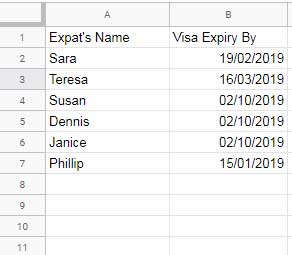
  
• In Sheet2, you have a shorter list of employee names in Column A.
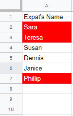
• You want to highlight the names in Sheet2!A:A only if their visas are expiring on or before a specific date (e.g., 31st March 2019).

Formula

Use this conditional formatting formula in Sheet2!A:A:

=COUNTIFS(INDIRECT("Sheet1!A:A"), A1, INDIRECT("Sheet1!B:B"), "<=" & DATE(2019, 3, 31))

Explanation

• INDIRECT("Sheet1!A:A"): Looks for a match of the name in Sheet1!A:A.
• A1: Refers to the current cell in Sheet2 being evaluated.
• INDIRECT("Sheet1!B:B"): Checks the corresponding visa expiry date in Sheet1!B:B.
• "<=" & DATE(2019, 3, 31): Adds the date condition to highlight only those names whose visa expires on or before March 31, 2019.
• COUNTIFS(...): Returns a count. If it’s 1 or more, it means both conditions are met and formatting will be applied.

Steps to Apply

1. Select the range in Sheet2!A:A.
2. Go to Format > Conditional formatting.
3. Choose Custom formula is.
4. Enter:
   =COUNTIFS(INDIRECT("Sheet1!A:A"), A1, INDIRECT("Sheet1!B:B"), "<=" & DATE(2019, 3, 31))
5. Pick a highlight color and click Done.

Summary

Using INDIRECT with XMATCH or COUNTIFS, you can easily highlight matching data across sheets in Google Sheets — with or without extra conditions like dates or status flags.

Related Resources

• Compare Two Google Sheets Cell by Cell and Highlight Differences
• Conditional Formatting Duplicates Across Tabs in Google Sheets