Ever missed a payment or forgotten a recurring event just because it wasn’t marked clearly in your spreadsheet? I’ve been there too. Thankfully, Google Sheets makes it super easy to automatically highlight recurring dates using a bit of Conditional Formatting magic.

In this post, I’ll show you exactly how to highlight recurring payment or event dates—whether they repeat every 14 days, monthly, or every two months—starting from a specific date (like 28 July 2021, which we’ll use in the example).

Let’s walk through this step-by-step.

Why Highlight Recurring Dates in Google Sheets?

Highlighting helps you stay organized and avoid nasty surprises like missed payments, forgotten subscriptions, or late fees. Here’s why I find it helpful:

• It keeps important dates visible at a glance
• It automates reminders without extra apps
• It works great for bills, subscriptions, gym memberships, or team meetings

And the best part? You can make your spreadsheet smart enough to highlight these dates automatically.

How Can You Highlight Cells in Google Sheets?

There are several ways to make certain cells stand out. You can:

• Draw a bold border
• Increase the font size
• Use a background fill color ✅
• Make text bold, italic, or underlined ✅
• Change the text color ✅

For recurring events or payments, I recommend using Conditional Formatting with background color and bold text for quick visibility.

Highlight Recurring Dates Every 14 Days (Biweekly)

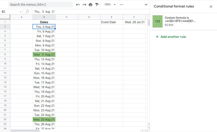
Let’s say you signed up for a gym membership or a biweekly subscription that started on 28 July 2021 (entered in cell F1), and now you want to highlight all the dates in column B that fall every 14 days from that start date.

The formula to use:

=AND(B2<>"", MOD(B2 - $F$1, 14) = 0)

What this does:

• Checks if the number of days between the date in B2 and the start date in F1 is a multiple of 14.
• If yes, it highlights that cell.

This means 11 Aug 2021, 25 Aug 2021, 8 Sept 2021, etc., would all be highlighted.

Highlight Dates That Repeat Every N Months

Let’s take it a step further. Maybe you have an event or payment that happens every two months instead. For instance, a bimonthly insurance premium that started on 28 July 2021.

Use this formula:

=AND(B2<>"", MOD(DATEDIF($F$1, B2, "M"), 2) = 0, DAY($F$1) = DAY(B2))

How it works:

• DATEDIF calculates how many full months have passed since your start date.
• MOD(..., 2) = 0 checks if it’s every second month.
• DAY(...) ensures the dates align on the 28th of each due month.

With this rule, dates like 28 Sept 2021, 28 Nov 2021, 28 Jan 2022 would be highlighted.

How to Apply These Rules in Google Sheets

Here’s how to bring it all together:

1. Select your range of dates in column B (e.g., B2:B1000).
2. Go to Format > Conditional formatting.
3. Under “Format cells if”, choose “Custom formula is”.
4. Paste in one of the formulas above.
5. Choose a background color (I like green for payments).
6. Click Done.

You can add multiple rules if you’re tracking more than one recurring item.

Can I Track Multiple Recurring Events?

Absolutely! Let’s say:

• You have one event every 14 days from F1 (28 July 2021)
• Another every two months from F2 (say, 5 August 2021)

Here’s how you’d set it up:

Rule for the 14-day cycle:

=AND(B2<>"", MOD(B2 - $F$1, 14) = 0)

Rule for the 2-month cycle:

=AND(B2<>"", MOD(DATEDIF($F$2, B2, "M"), 2) = 0, DAY($F$2) = DAY(B2))

Just assign a different color to each rule so you can easily tell them apart. This makes it super flexible for managing multiple schedules within the same sheet.

A Few Things to Note

• Your dates can be in any order. The formula still works.
• You don’t need to list all dates manually—just enough to cover the year or planning period.
• You can tweak the frequency: Change 14 to 7 for weekly, or 2 to 1 for monthly.

Resources

• How to Highlight Cells Based on Expiry Date in Google Sheets
• Create a Dynamic Date That Advances or Resets in Google Sheets
• Get the Next Renewal Date Based on Custom Month Intervals
• Find Next Biannual, Annual, Biennial, and Triennial Dates
• Date-Related Conditional Formatting Rules in Google Sheets