


")


")

")
")
 in Excel & Google Sheets")


If you want to highlight filtered output from a formula in Google Sheets, here’s a neat trick using ROW and XMATCH along with your existing FILTER formula.
This method has two big advantages:
- You can highlight the matching rows in your source table instead of filtering them out, which normally makes the result uneditable. This way, you can update data directly in the original range without breaking any formulas.
- It saves time when applying filters across multiple columns. Instead of using Data > Create a filter again and again, you can just highlight the matching rows and then use Filter by color. Simple and visual.
Is It Difficult to Highlight Filtered Output in Google Sheets?
Not at all. If you already have a FILTER formula, you’re more than halfway there. You just need to tweak it slightly to build a conditional formatting rule that highlights the same filtered output — right inside the original range.
Sample Data and Filter Setup
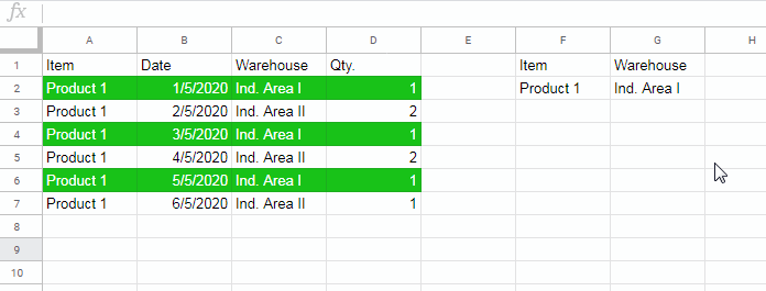
Let’s say your data is in columns A to D:
- Column A – Item names
- Column B – Date
- Column C – Storage yard
- Column D – Quantity
We’ll filter rows based on these two conditions:
- Item in column A is
"Product 1" - Storage yard in column C is
"Ind. Area II"
When these conditions match, the corresponding rows in the source table should be highlighted.
And if you later change the condition in cell G2 to "Ind. Area I", the highlighting should update automatically.
How to Highlight Filtered Output from a Formula
Let’s go step-by-step.
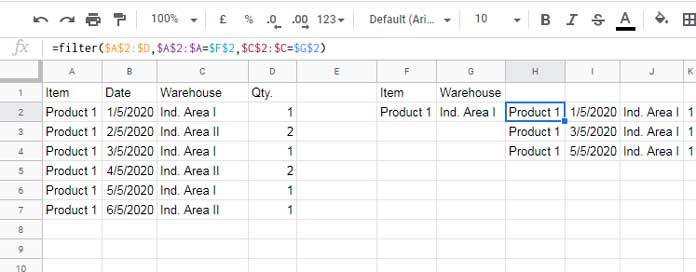
Step 1: Your Original FILTER Formula
Here’s the formula that filters the table based on two criteria:
=FILTER($A$2:$D, $A$2:$A = $F$2, $C$2:$C = $G$2)$F$2contains the product name$G$2contains the storage yard name
Make sure you use absolute references (with $ signs), especially if you’re using this inside a formatting rule.
Step 2: Get the Row Numbers of the Filtered Results
This is the key trick. Instead of returning the actual rows from the table, let’s return their row numbers:
=FILTER(ROW($A$2:$D), $A$2:$A = $F$2, $C$2:$C = $G$2)You’ll get something like:
3
5
7
Those are the row numbers where the conditions are met.
Step 3: Write the Conditional Formatting Formula
Now let’s build a formula that checks whether the current row is in the list above.
This is what you’ll use inside the conditional formatting rule:
=XMATCH(ROW(A2), FILTER(ROW($A$2:$D), $A$2:$A = $F$2, $C$2:$C = $G$2))This returns a number if the row is found in the filter result, or an error if it isn’t. Conditional formatting treats any number as TRUE, so only matching rows will be highlighted.
Step 4: Apply the Conditional Formatting
- Select your source range — for example,
A2:D - Go to Format > Conditional formatting
- Under “Format rules,” choose Custom formula is
- Paste the formula from Step 3
- Pick your highlight color
- Click Done
That’s it — your table now highlights only the rows that match the filter conditions in F2 and G2.
Change either condition, and the highlighting will adjust automatically.
Bonus Tip: Filter by Color
Once the filtered rows are highlighted, you can use Filter by color to quickly isolate and work with just those rows — no need to create new filters.
Here’s how:
- Click anywhere in the data range (e.g., column A)
- Go to Data > Create a filter
- Click the filter dropdown in the header
- Choose Filter by color > Fill color and select your highlight color
Now you’ll see only the highlighted rows — and you can freely edit them without touching the formula.
Remember: if you change the condition in F2 or G2, you’ll need to come back here and apply Filter by color again. The highlighting updates automatically, but the filter by color doesn’t adjust until you reapply it.
Conclusion
This is one of my favorite ways to highlight filtered output in Google Sheets without losing the flexibility to work with the data. It’s quick, visual, and avoids the formula-breaking frustrations of editing a filtered result directly.