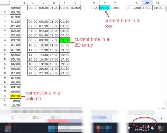
Do you want to automatically highlight the cell or the entire row or column containing the current time in Google Sheets? We’ve got you covered.
Typically, you may have a column containing a sequence of time intervals, such as 15 minutes, 30 minutes, or 1 hour.
In this context, highlighting the current time doesn’t always refer to the exact current time, but rather to matching the time interval that falls on or just before the current time.
We want to create a highlight rule that uses a combination of functions.
Highlighting the Current Time Cell (Rows or Columns)
In this, we will focus on a highlight rule that automatically highlights a cell in a range matching the current time.

Here are the step-by-step instructions:
- Select the range of cells containing the time sequence. This range can be one-dimensional, like A1:A (vertical) or C1:1 (horizontal), or two-dimensional, like C4:F15.
- Click on the Format menu and select Conditional Formatting.
- If you already have a rule in the selected range, click the Add Another Rule button. Otherwise, proceed to the next step.
- Under Format Rules, select Custom Formula from the drop-down menu.
- Copy and paste the following formula:
=XMATCH(FLOOR(MOD(NOW(), 1), "0:30"), A1). Replace A1 with the reference of the first cell in the range to highlight. Then, replace “0:30” with the time interval present in your range to highlight. For example, for 15 minutes, specify it as “0:15”, and for a 1-hour interval, specify it as “1:00”. - Under Formatting Style, select your choice of highlighting.
- Click Done.
This way, you can automatically highlight the current time in a cell within a row, column, or 2D array in Google Sheets.
Formula Breakdown
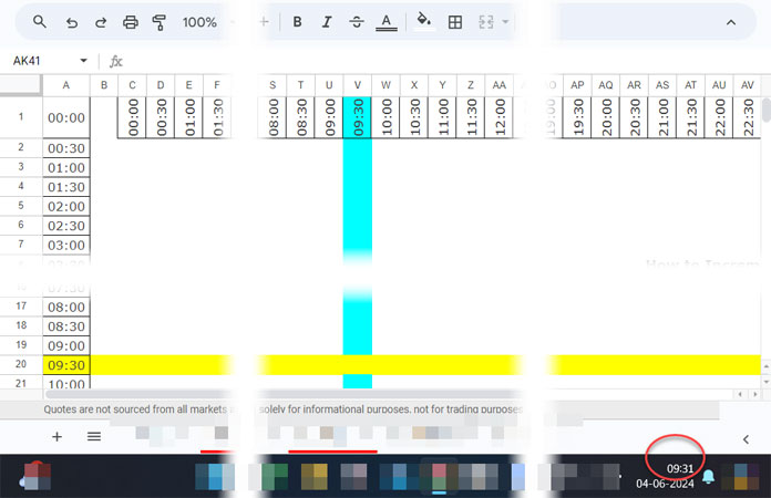
This is an all-weather formula. You can easily modify it to match the current time in a row or column and highlight that entire row or column in Google Sheets.
First, we will understand the formula, and then proceed to that simple modification in the next section.
NOW(): The NOW function returns the current date and time.MOD(…, 1): The MOD function returns the remainder after division. When you divide a datetime by 1, the remainder will be the time component.FLOOR(…, "0:30"): The FLOOR function rounds down the time to the nearest integer multiple of the factor, the time interval.=XMATCH(..., A1): The XMATCH function matches this value in each cell in the selected range, forming the conditional format rule to highlight the current time, which auto-refreshes within the applied range.
Match the Current Time and Highlight the Entire Row or Column
This section discusses how to automatically highlight an entire row or column that matches the current time in that respective row or column.

Assume you want to match the current time in A1:A, and the formula finds it in A20. You want to highlight row #20.
You need to make only one change in the formula. Replace A1 (relative reference) in the formula with $A1 (column absolute, row relative).
Please replace the “Apply to range” in the Conditional Format Rules panel with A1:Z, or from A1:A to the column you want.
Similarly, to match the current time in C1:1 and highlight the entire column, replace A1 (relative reference) with C$1 (column relative, row absolute).
Here also apply the rule to the range (“Apply to range”) something like C1:100 or from C1:1 to the row you want.
Resources
Here are some related resources in Google Sheets that discuss time sequences and conditional formatting based on dates.
- How to Increment Time By Minutes and Hours in Google Sheets
- How to Increment DateTime by One Hour in Google Sheets (Array Formula)
- Create Custom Time Slot Sequences in Google Sheets
- How to Highlight Cells Based on Expiry Date in Google Sheets
- Highlight Earliest Events Based on Date Column in Google Sheets
- How to Highlight Recurring Events or Payment Dates in Google Sheets
- Date-Related Conditional Formatting Rules in Google Sheets


