The FALSE function in Google Sheets returns the Boolean value FALSE. But you don’t always need to use this logical function to get the Boolean value. Google Sheets automatically recognizes the word FALSE (not case-sensitive) as the Boolean value in most situations.

There are several ways to enter the Boolean FALSE value in a cell or formula:

• Simply type FALSE (case-insensitive) in a cell
• Use the formula =FALSE
• Or use the function =FALSE()

When you need to specify FALSE in a formula as a criterion or argument, you can use either FALSE or FALSE() — both work the same.

Note: In QUERY functions, only the first method (FALSE without parentheses) works.

Why Both FALSE and FALSE() Exist?

• FALSE is treated as a Boolean constant, like a keyword.
• FALSE() is a function that returns the same constant.

They are functionally equivalent in almost all use cases.

Syntax of the FALSE Logical Function

The FALSE function in Google Sheets has no arguments:

FALSE()

It simply returns the Boolean FALSE.

How to Use the FALSE Function in Google Sheets

Example 1: Return FALSE if a Logical Expression is False

=A1=20

This formula will return TRUE if the value in cell A1 is 20; otherwise, it returns FALSE.

Here’s the equivalent formula using an IF statement:

=IF(A1=20, TRUE, FALSE)

You can also replace TRUE with TRUE() and FALSE with FALSE() as shown below:

=IF(A1=20, TRUE(), FALSE())

Example 2: Filter Rows Where Values Are Boolean FALSE

This example shows how to use the FALSE function in Google Sheets to filter datasets:

=FILTER(A2:B, B2:B=FALSE)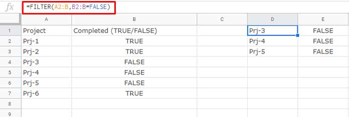

You can also write it using the FALSE() function:

=FILTER(A2:B, B2:B=FALSE())

Both formulas return the same result.

But in a QUERY formula, you cannot use FALSE() — only the plain FALSE (without parentheses) works. This is because the condition is written as a text string inside the query, and FALSE is recognized as a keyword within that string, not a function.

=QUERY(A2:B, "SELECT A, B WHERE B=FALSE")

If you try to use FALSE() inside the query string, it won’t be parsed correctly since the query language (based on SQL) does not understand spreadsheet functions like FALSE() — it expects FALSE as a literal keyword.

Additional Tips

• To convert FALSE to 0 and TRUE to 1, wrap the value in the N function:
  =N(A1)
  If cell A1 contains FALSE, this will return 0.
• You can format cells containing the FALSE value as tick boxes. Select the cells, then go to Insert > Tick box. The FALSE value will become an unchecked tick box that you can toggle. If the cell contains the FALSE() function, you can still format it as a tick box — but you won’t be able to manually toggle it.