Google Sheets: Extract Top N per Group from Query Aggregation

When working with grouped and aggregated data in Google Sheets, you might need to extract the top N values within each group rather than from the entire dataset. While the QUERY function is excellent for summarizing data by groups, it doesn’t provide a built-in way to filter the highest values within each category.

Although you can limit the number of rows in the result using the LIMIT clause in QUERY, it does not apply group-wise filtering.

How to Extract Top N per Group from Query Aggregation

To extract top N per group from QUERY aggregation, use the following formula:

=ArrayFormula(
   LET(
      qry, QUERY(QUERY(data, "SELECT Col2, Col1, SUM(Col3) WHERE Col2 IS NOT NULL GROUP BY Col2, Col1 ORDER BY Col2, SUM(Col3) DESC", 1), "OFFSET 1", 0), 
      rnk, COUNTIFS(CHOOSECOLS(qry, 1), CHOOSECOLS(qry, 1), CHOOSECOLS(qry, 3), ">"&CHOOSECOLS(qry, 3))+1, 
      FILTER(qry, rnk<=n)
   )
)

Formula Components:

Replace data with the three-column dataset, where:
- Column 1: Item
- Column 2: Category (e.g., location)
- Column 3: Values to sum
Replace n with the number of top values to extract per group. For example:
- Use 3 to extract the top 3 items per group.
- Use 10 for the top 10 items per group.

The formula follows Excel Pivot Table’s tie-breaking method—it extracts the top N items in each group and includes any additional items that share the Nth value.

For example, if the aggregated values within a group are {42, 42, 16, 16, 10, 8}, extracting the top 3 will return 42, 42, 16, 16 (including ties).

Example: Extracting Top N per Group from Query Aggregation

Sample Data:

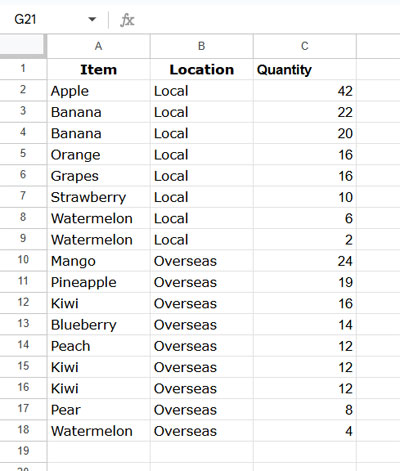
We will extract the top 3 best-selling fruits in both Local and Overseas markets.

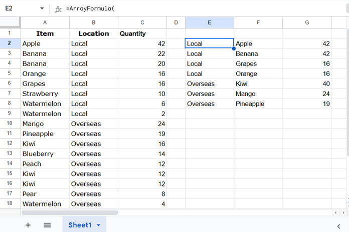
Formula to Extract the Top 3 Per Group:

=ArrayFormula(
   LET(
      qry, QUERY(QUERY(Sheet1!A1:C, "SELECT Col2, Col1, SUM(Col3) WHERE Col2 IS NOT NULL GROUP BY Col2, Col1 ORDER BY Col2, SUM(Col3) DESC", 1), "OFFSET 1", 0), 
      rnk, COUNTIFS(CHOOSECOLS(qry, 1), CHOOSECOLS(qry, 1), CHOOSECOLS(qry, 3), ">"&CHOOSECOLS(qry, 3))+1, 
      FILTER(qry, rnk<=3)
   )
)

data: Sheet1!A1:C
n: 3 (can be changed to 5, 10, etc.)

Example of extracting top N per group from query-aggregated data in Google Sheets

To extract the top 5 per group, replace 3 with 5. To extract the top 10, replace 3 with 10.

How This Formula Works

Understanding the formula logic helps you customize and optimize it for different use cases.

Step-by-Step Breakdown

1. Aggregate and Sort Data

QUERY(Sheet1!A1:C, "SELECT Col2, Col1, SUM(Col3) WHERE Col2 IS NOT NULL GROUP BY Col2, Col1 ORDER BY Col2, SUM(Col3) DESC", 1)

Groups the data first by Location (Col2) and then by Item (Col1).
Aggregates the Quantity (SUM(Col3))
Sorts by Location (ascending) and Quantity (descending) to keep the top values at the top

2. Remove Header Row

QUERY(..., "OFFSET 1", 0)

Removes the header row from the query output

3. Rank the Aggregated Values Within Each Group

COUNTIFS(CHOOSECOLS(qry, 1), CHOOSECOLS(qry, 1), CHOOSECOLS(qry, 3), ">"&CHOOSECOLS(qry, 3))+1

Computes the rank of each aggregated value within its group

4. Filter the Top N per Group

FILTER(qry, rnk<=3)

Extracts the top N items per group by filtering the highest-ranked values

This is how you can efficiently extract top N per group from QUERY aggregated results in Google Sheets using a dynamic, formula-based approach.