The CELL function helps us gather specific information about a cell or the top-left cell in a range, allowing us to make informed decisions in Google Sheets.

What kind of information can we retrieve from a cell using this function, and how can it be useful? Let’s explore that in this Google Sheets tutorial.

Syntax

CELL(info_type, reference)

• info_type – The type of information you want to retrieve.
• reference – You refer to a cell or cell range. If you refer to a cell range, the function considers only the first (top-left) cell.

Here are two examples of the CELL function in Google Sheets:

• =CELL("col", Z10) // returns 26, the column number of cell Z10
• =CELL("col", A2:C100) // returns 1, the column number of the top-left cell (A2) in the range A2:C100.

Understanding the Info Types in the CELL Function

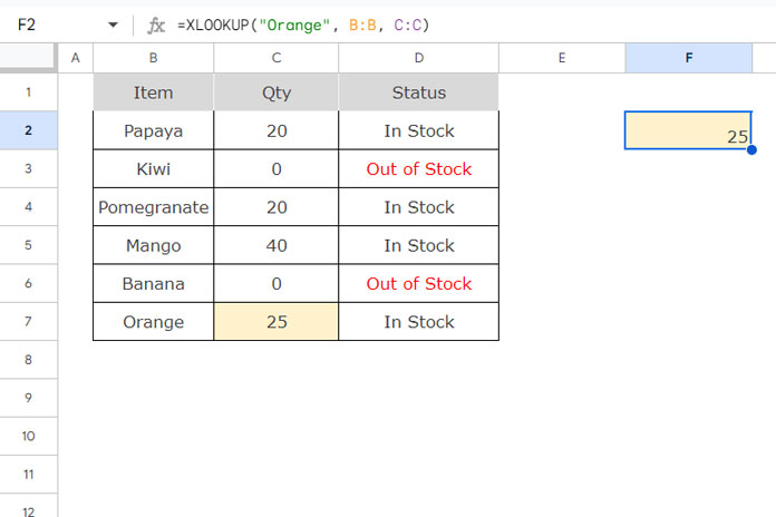
Assume you have a table with product names in column B, available quantities in column C, and status in column D.

Look up a product and gather information using the CELL function.

We will use the feature-packed XLOOKUP function for the lookup.

=XLOOKUP("Orange", B:B, C:C)

This formula looks up “Orange” in column B and returns the corresponding quantity from column C.

Now, let’s use different CELL function info types to gather additional details about the cell where this quantity is located.

Examples:

In the following examples, we will use various info types available in the CELL function one by one.

• =CELL("address", XLOOKUP("Orange", B:B, C:C))
  Returns $C$7, the cell address of the XLOOKUP result cell.
• =CELL("col", XLOOKUP("Orange", B:B, C:C))
  Returns 3, the column number of the result cell.
• =CELL("row", XLOOKUP("Orange", B:B, C:C))
  Returns 7, the row number of the result cell.
• =CELL("type", XLOOKUP("Orange", B:B, C:C))
  Returns “v”, the type of the result.
  Types are:
  • “b” for a blank cell
  • “l” for a label (plain text)
  • “v” for a value or any other data type such as date, time, or timestamp.
• =CELL("prefix", XLOOKUP("Orange", B:B, C:C))
  Returns the horizontal alignment of the value. The output here will be “^” since the result cell is center-aligned. Text alignments are represented as follows:
  • A single quotation mark (‘) for left-aligned values
  • A double quotation mark (“) for right-aligned values
  • A caret (^) for center-aligned values
  • Blank if the cell is empty

Other Info Types:

• “color” – Returns 1 if the cell is formatted to display red for negative numbers; otherwise, returns 0. To test this, go to cell E1, click Format > Number > Custom Number Format, and enter the format #,##0_);[Red](#,##0) . Then, try =CELL("color", E1).
• “contents” – Returns the value in the referenced cell.
• “width” – Returns the width of the column in terms of the number of characters. Each unit is equal to the width of the zero (0) character in the default font size.

Important: I noticed that two of the info types in the CELL function, namely prefix and width, do not refresh when the cell information changes. For example, if =CELL("width", XLOOKUP("Banana", B:B, C:C)) returns 13, it will remain the same even after you change the width. To get the updated width, you should reapply the formula (copy it, delete it, and then paste it again).

Using the CELL Function in Conditional Formatting

The following example will help you understand how useful the CELL function can be in Conditional Formatting.

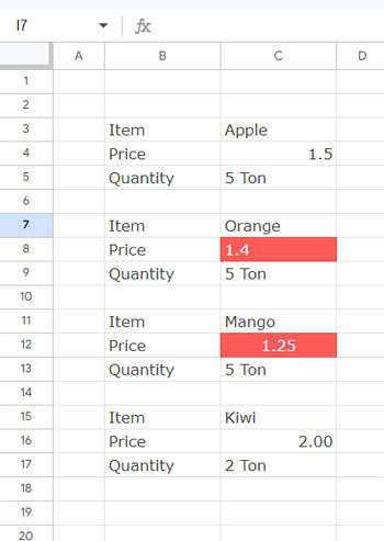
Suppose you have a column of data that includes both numbers and text. If you want to ensure all numbers are right-aligned, you can use the following highlight rule.

If the column is C, you can use the following formula:

=AND(ISNUMBER(C1), OR(CELL("prefix", C1)="'", OR(CELL("prefix", C1)="^")))

To apply this rule, select column C, then click Format > Conditional Formatting. In the sidebar panel that opens, select “Custom formula is” under Format Rules. Enter the formula above and click Done.

Explanation of the formula:

• ISNUMBER(C1): Returns TRUE if the content of the cell is numeric.
• OR(CELL("prefix", C1)="'", CELL("prefix", C1)="^"): Returns TRUE if the cell is aligned left (denoted by a single quotation mark) or center (denoted by a caret).

The AND function returns TRUE if both of the above conditions are met, and those cells will be highlighted.

Note: The highlighting will not reflect any changes made to the cell after you apply the rule.

Using the CELL Function in Data Validation

Do you want to require users to enter values only in a center-aligned column?

You can use the CELL function to create a suitable data validation rule.

Let’s consider column C for this test.

1. Select column C and click on Data > Data Validation.
2. Click the “+ Add Rule” button.
3. Select “Custom Formula Is” under Criteria.
4. Enter =CELL("prefix", C1)="^".
5. Under Advanced Options, select Reject Input.
6. Check “Show help text for a selected cell” and enter: “Center-align the column (horizontal alignment).”
7. Click Done.

Users will need to center-align the column to enter values.