We can use a formula or a named function to calculate the next renewal date of a subscription model, specified in n months, in Google Sheets.

The easiest way is to use the Map lambda function because it will help us to renew all dates in a column in one go!

Assume we have given maintenance contracts to several parties for a given period.

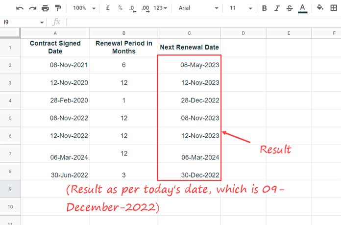
In a Sheet, we have a column (field) titled “Contract Signed Date,” which contains all our maintenance contract-signed dates with different parties.

The next column (field) is titled “Renewal Period in Months,” in which we can specify the contract auto-renewal period in months.

For example, we signed a maintenance contract in 28-Feb-2020. It should be auto-renewed every 12 months.

Today is 09-Dec-2022. So the next renewal date of the above contract must be 28-Feb-2023.

Next Renewal Date: Sample Data, Formula, and Explanation

In the following example, the data is in columns A and B.

My formula finding the next renewal date is in cell C2, which spills down provided C3:C blank.

It’s a lengthy formula based on the relatively new Map function. But the logic behind it seemed to be easy to learn.

You May Like:- Google Sheets Function Guide.

Here is the formula to find the next renewal date in Google Sheets.

Master Formula:

=ifna(
   map(
      A2:A,B2:B,
         lambda(
            cs,rp,
               if(cs>today(),
                  cs,
                  index(
                     filter(
                        edate(cs,sequence(datedif(min(A2:A),today(),"m")+1,1,rp,rp)),
                        edate(cs,sequence(datedif(min(A2:A),today(),"m")+1,1,rp,rp))>today()
                     ),1
                  )
               )
         )
   )
)

Note 1:- The result will be date values. So you must select the range C2:C8 and apply Format > Number > Date.

The above formula is not so complex. Please go through the formula explanation below. I’m sure you will be blown away by its simplicity.

Formula Logic and Explanation

Logic:

Using the EDATE function, we can find a date that is a specified number of months before (-ve months) or after (+ve months) another date.

Syntax: EDATE(start_date, [months])

E.g.:

=edate("08/11/2021",6)

Where start_date is 08/11/2021 (contract signed date) and the months is 6 (renewal period in months). So, the above EDATE formula will return the date 08/05/2022.

When we replace 6 (months) with multiples of 6, such as 6, 12, 18, 24, etc., the formula will return multiple dates.

=ArrayFormula(edate("08/11/2021",{6;12;18;24;30}))

Result: 08/05/2022, 08/11/2022, 08/05/2023, 08/11/2023, and 08/05/2024.

Note 2:- When specifying multiple months, we must use the ArrayFormua function.

How does this formula fit into our purpose of finding the next renewal date in Google Sheets?

Using the FILTER function, we can filter out past dates.

=filter(edate("08/11/2021",{6;12;18;24;30}),edate("08/11/2021",{6;12;18;24;30})>today())

Note 3:- The ArrayFormula function is not required within the Filter formula.

Result: 08/05/2023, 08/11/2023, and 08/05/2024.

We can get the first date from this filtered result using the INDEX function.

Basic Formula:

=index(filter(edate("08/11/2021",{6;12;18;24;30}),edate("08/11/2021",{6;12;18;24;30})>today()),1)

The result will be a date value. Format that to date and that will be our next renewal date.

So the logic is to generate a list of renewal dates, filter out past dates and get the upcoming one from the list.

Customizing the Basic Next Renewal Date Formula

We must make a few changes before using the above basic next renewal date formula.

In the master formula, we used cell references. Let’s modify the above accordingly.

=index(filter(edate(A2,{6;12;18;24;30}),edate(A2,{6;12;18;24;30})>today()),1)

The next step is to replace {6;12;18;22;28} with multiples of B2 and the equivalent is sequence(5,1,B2,B2).

=index(filter(edate(A2,sequence(5,1,B2,B2)),edate(A2,sequence(5,1,B2,B2))>today()),1)

If you check the renewal period in column B, you can find that the renewal period is not always every six months. There is one month, three months, and one-year (12 months) renewals.

So using 5 (number of multiples) won’t always work.

The ideal way is to find the total number of months between the contract signed date and today’s date and +1 month.

So replace 5 with datedif(A2,today(),"m")+1.

=index(filter(edate(A2,sequence(datedif(A2,today(),"m")+1,1,B2,B2)),edate(A2,sequence(datedif(A2,today(),"m")+1,1,B2,B2))>today()),1)

We have used the MAP lambda helper function to fill this formula down. While doing so, we replaced A2 in the above DATEDIF with min(A2:A).

Note 4:- The formula might have performance issues if it finds a long past “contract signed date” (more than ten years old) in column A.

Custom Named Function to Get the Next Renewal Date

For ease of use, I’ve converted the above formula to a Named Function. Here it is.

Syntax: NEXT_RENEWAL_DATE(array1, array2)

array1 – The cell or array that contains the contract signed/subscription date.

array2 – The cell or array that contains the contract renewal period/subscription model in months.

Examples:

1. Subscription Date is 08/11/2021 and the subscription model is every six months.

=NEXT_RENEWAL_DATE(date(2021,11,8),6)

2. If you enter the date in A2 and period in B2, you can use the NEXT_RENEWAL_DATE formula as follows.

=NEXT_RENEWAL_DATE(A2,B2)

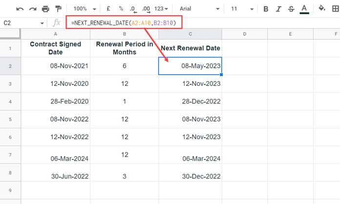
3. If you use a range, as per our earlier screenshot, the formula will be as follows.

=NEXT_RENEWAL_DATE(A2:A10,B2:B10)

Function Import:- To import the above function, please make a copy of the following file and import from it.

Named Function 091222

That’s all. Thanks for the stay. Enjoy!