This is a beginner’s guide on how to use Freeze Panes in Google Sheets. I’ll explain the concept of Freeze Panes with screenshots.
While it’s easy to freeze rows or columns in Google Sheets, understanding its importance will help you maximize its utility. Freeze Panes in Google Sheets is not just for freezing rows or columns—it can also be used to set headers in print formats.
I have several medium to advanced-level tutorials related to Google Sheets on this page. However, I realized that I was missing some basic tutorials. Initially, I skipped over Google Sheets beginners’ tips because I assumed most users were transitioning from Excel or similar spreadsheet applications. But I’ve come to realize that many people are new to spreadsheets altogether. So, this tutorial is aimed at helping such users. Let’s get started!
What is Freeze Panes?
Freeze Panes refers to keeping specific rows or columns visible while you scroll through the rest of your spreadsheet. This is useful when you want to keep titles or important information visible, regardless of how far down or across you scroll. Once you freeze a row or column, it stays in place until you unfreeze it.
How to Set Freeze Panes in Google Sheets
I’ve divided this tutorial into five sections:
- How to Freeze Rows in Google Sheets
- How to Freeze Columns in Google Sheets
- How to Freeze Rows and Columns Together in Google Sheets
- Unfreeze Columns / Rows
- How to Use Freeze Panes for Headers or Page Titles in Google Sheets
Let’s go through them one by one.
How to Freeze Rows in Google Sheets
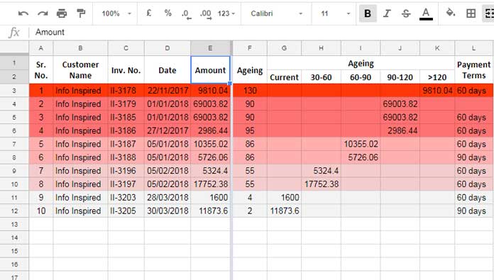
For demonstration, I will use one of my custom heat map files. In this example, certain cells in the first two rows are merged. These rows contain the titles for my heat map.
To freeze these two rows (so they stay visible when you scroll down), follow the below step:
- Go to the menu: View > Freeze > 2 rows (as shown in the screenshot).

Google Sheets will automatically suggest freezing up to the row where your active cell is located. For example, if your active cell is in row 6, the suggestion will be “Up to row 6” in the View menu under Freeze.
How to Freeze Columns in Google Sheets
You can also freeze columns in Google Sheets. Though less common than freezing rows, it can still be useful. To freeze a specific column:
- Navigate to any cell in the column you want to freeze (e.g., column E).
- Go to View > Freeze > Up to column E.
The dark shaded line indicates where the Freeze Pane starts.

How to Freeze Rows and Columns Together in Google Sheets
Freezing both rows and columns together requires two steps. You can’t do this in one click, but it’s simple:
- First, freeze the rows as described above.
- Then, freeze the columns following the steps for freezing columns.
For example, here are the steps I followed:
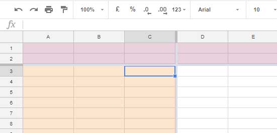
- My active cell was C3.
- View > Freeze > Up to column C
- View > Freeze > 2 rows

How to Unfreeze Columns / Rows in Google Sheets
To unfreeze any rows or columns, go to the View > Freeze menu, and select No rows or No columns.
The Role of Freeze Panes for Headers in Google Sheets
If you have a large Google Sheets document with many rows, the data may spread across multiple pages when printed. You might want the first row (or a few rows) to repeat at the top of each page as header rows—especially if your first row contains field labels.
To make sure your titles or headers repeat on every printed page, freeze the rows that you want to appear at the top. This will allow them to act as print titles.
For more information on setting print titles in Google Sheets, you can refer to my post: How to Add Repeat Page Titles in Google Sheets.
Important Notes
You can place images, drawings, and pivot tables over cells within the frozen panes. They will remain visible when you scroll down or to the right.
However, at present, you cannot place a chart within the frozen panes.


