Many Google Sheets users face challenges when working with time durations that include milliseconds. This is often due to incorrect time formatting. To solve this issue, you must first understand how to format time to include milliseconds in Google Sheets.
In Google Sheets, milliseconds are separated from the seconds field by a dot (.), not a colon (:). If you don’t follow the correct format, the spreadsheet might interpret the entered time as text instead of a valid time value.
The Incorrect Way to Enter Time in Millisecond Format in Sheets
10:45.360
This is an incorrect format. Google Sheets will treat this as a text string. In the example above, the time is entered in the mm:ss.000 format, which is not valid.
Tip: If you’ve already entered time as text (like in the example), you can fix it with a formula workaround. I’ll explain this later in the tutorial.
The Correct Way to Enter Time in Millisecond Format in Sheets
00:10:45.360
This is the correct format. You must include the hours in the format. The correct format is hh:mm:ss.000. Only then will Google Sheets recognize the value as time. However, there is one issue!
While this format ensures the value is treated as time, the milliseconds might be rounded and not visible. You’ll need to adjust the formatting to display them.

Below, I explain how to format time values to display milliseconds in Google Sheets.
Steps to Format Time to Milliseconds in Google Sheets
Now that you know how to correctly enter milliseconds in Google Sheets, the next step is to format the time so that the milliseconds are displayed.
Steps:
- Select the cell containing the time entered in the
hh:mm:ss.000format. - Go to the menu: Format > Number > Custom number format.
- In the field, enter the format
hh:mm:ss.000and click Apply.
This will format the time or duration to include milliseconds in Google Sheets.

Fixing Time Entered as Text
If you’ve entered time in the mm:ss.000 format (treated as text), it can’t be used in time calculations. You can correct this in two ways.
1. Manually Correct Time Text Entries
If there are only a few cells, you can manually edit them. For example:
- Assume cell
A1contains45:26.148(text). - Edit it to
00:45:26.148. - Then, use the format menu as explained earlier to display the milliseconds.
2. Bulk Convert mm:ss.000 Text to hh:mm:ss.000 Time Format
For multiple cells, use a formula to make corrections.
Example:
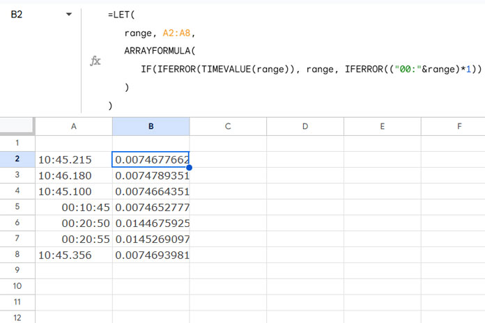
Assume time values are in the range A2:A8. This range may contain a mix of text-formatted durations and actual time durations. Enter the following formula in cell B2:
=LET(
   range, A2:A8,
   ARRAYFORMULA(
      IF(IFERROR(TIMEVALUE(range)), range, IFERROR(("00:"&range)*1))
   )
)
This formula:
- Adds
00:to the beginning of each text value inA2:A8and converts it to a numeric time value. - Retains the original durations for cells already formatted as valid times.

When you use this formula, simply replace A2:A8 with the desired range in your sheet.
How the Formula Works:
- The IF function evaluates
IFERROR(TIMEVALUE(range)).- If the cell contains a valid time value, it is retained as is.
- If the cell contains text, the formula applies
IFERROR(("00:" & range) * 1)to convert the text to a time value.
This approach ensures all values in the range are properly formatted for calculations while preserving existing time entries.
Steps to Apply the Corrected Time Format:
- Select the formula output range (e.g.,
B2:B8) and copy it. - Right-click on cell
A2, then choose Paste Special > Values Only. - Select the range
A2:A8and apply the formathh:mm:ss.000as explained earlier. - Delete the formula in
B2.
That’s it!
Summary of Tips Learned
In this quick Google Sheets tutorial, you’ve learned:
- How to format time to include milliseconds in Google Sheets.
- How to convert text-formatted time values to valid time with milliseconds.
If you found this helpful, feel free to share! Thanks for reading.
More Resources
- How to Remove Milliseconds from Timestamps in Google Sheets
- How to Convert a Timestamp to Milliseconds in Google Sheets
- How to Plot a Line Chart Using Lap Times in Milliseconds
- Comparing Timestamps and Standard Dates in Google Sheets
- Extracting Date From Timestamp in Google Sheets: 5 Methods
- How to Automate Overtime Calculation in Google Sheets
- How to Convert Military Time to Standard Time in Google Sheets
- Elapsed Days and Time Between Two Dates in Google Sheets
- Countdown Timers in Google Sheets (Easy Way!)
- How to Add Hours, Minutes, Seconds to Time in Google Sheets


