Can we format a date from “DD/MM/YYYY” to “DD-MMM-YYYY” or any other format using a formula without converting it to text in Google Sheets?

My answer is “Yes.” We can format a date using a formula while keeping the underlying date value in Google Sheets.

Your search for a formula to format dates usually leads to a solution using the TEXT function, right? But is there an alternative to the TEXT function in Google Sheets to format a date?

Yes! Let’s dive into that. But first, let’s explore why the TEXT function may not always be the best option.

The Issue with Using the TEXT Function to Format Dates

The TEXT function has a significant limitation that you may have already encountered. Let’s test that and explore further.

In the following example, we will use the TEXT function to format a date from “DD/MM/YYYY” to “DD-MMM-YYYY”:

• Cell C2 contains the date 26/01/2023. It’s an original date in a recognizable date format. We can use the following formula in cell D2 to format this date:

=TEXT(C2, "DD-MMM-YYYY")

Now, let’s test the result of this formula.

Testing the Date Formatted Using the TEXT Function

We have our original date in cell C2 and the TEXT-formatted date in cell D2.

Here are the test results:

Notice the last formula, which returns FALSE instead of TRUE! Even though 31/12/2025 is greater than 26/01/2023, the formula returns FALSE.

You may face issues when using a TEXT-formatted date within functions such as ISBETWEEN, FILTER, etc., or wherever comparison operators are involved.

Here’s another example before we attempt to format a date using a formula for date formatting without text conversion.

Additional Example: Date Formatting Using TEXT

I’ve used =TEXT(C2, "DD-MMM-YYYY") in D2 and =TEXT(C3, "DD-MMM-YYYY") in D3 to format the dates in C2 and C3, respectively.

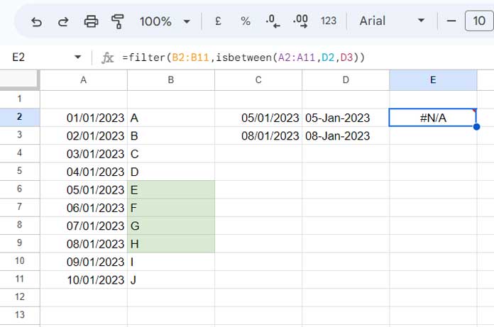
Formula #1:

=FILTER(B2:B11, ISBETWEEN(A2:A11, D2, D3))

I expect it to return “E,” “F,” “G,” and “H”—the values in the highlighted cells.

However, using Formula #1, we get an #N/A error.

Now, here’s the correct formula using the original dates:

Formula #2:

=FILTER(B2:B11, ISBETWEEN(A2:A11, C2, C3))

This one works correctly because it uses the original date values.

Formatting a Date Using a Formula Without Converting it Into Text

Now, let’s talk about the solution.

We can format a date using a formula without converting it into text in Google Sheets. This can be done using the QUERY function and the FORMAT clause.

For example, in the case where Formula #1 returns #N/A, we can apply the QUERY function as follows:

• In D2, enter:
  =QUERY(C2, "FORMAT C 'DD-MMM-YYYY'")
• In D3, enter:
  =QUERY(C3, "FORMAT C 'DD-MMM-YYYY'")

This will correctly format the date while keeping the underlying date value intact.

The QUERY function allows us to format the date without converting it to text, and Formula #1 will now work correctly.

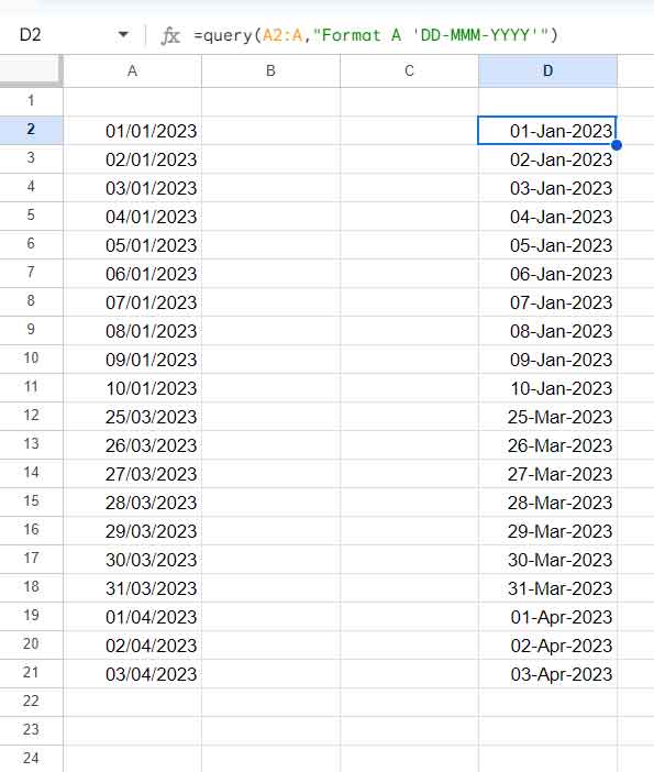
Formatting All Dates in Column A

What if you want to format all the dates in column A while keeping the underlying date values?

Here’s the formula for that:

=QUERY(A2:A, "FORMAT A 'DD-MMM-YYYY'")

This formula will format the entire column of dates without converting them into text.

Conclusion

In this post, we’ve learned how to use a formula for date formatting without text conversion in Google Sheets. By using the QUERY function with the FORMAT clause, you can format your dates in a custom way while maintaining their true date values, allowing you to use them effectively in further calculations or functions.

Resources

• Formatting Date, Time, and Numbers in Google Sheets Query
• Convert Text Dates with Dots to Slash Format in Google Sheets
• Combine Text and Date in Google Sheets Using Formula