


")


")

")
")
 in Excel & Google Sheets")


Finding and eliminating duplicates using the QUERY formula in Google Sheets involves creating a new range without duplicates.
To clarify, if you want to remove duplicates directly from the source data, Google Sheets already provides a built-in tool for that. If you prefer using formulas, you can employ functions like UNIQUE or SORTN depending on your needs.
What sets the QUERY approach apart, and when should you use it for duplicate removal?
Consider the table below, where columns A to D display items, area, quantity (Qty), and amount:
| Items | Area | Qty | Amount |
| Apple | North | 12 | 54 |
| Orange | South | 7 | 32 |
| Apple | North | 17 | 77 |
| Banana | East | 10 | 45 |
| Orange | South | 5 | 23 |
| Apple | West | 14 | 63 |
The goal is to remove duplicates from columns A (Items) and B (Area) while retaining the values from duplicate rows in other columns by summing them up in the retained row.
For example, for “Apple – North”:
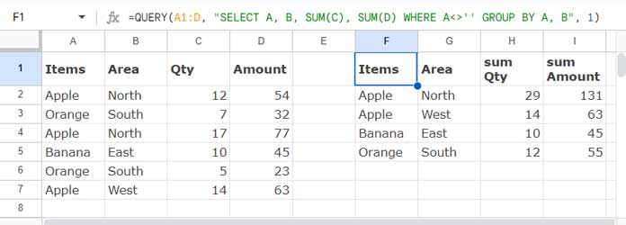
Combine quantities: 12 + 17 = 29
Combine amounts: 54 + 77 = 131
You can extract unique items and return the row with the minimum quantity, maximum quantity, or both using the QUERY function.
This comprehensive approach covers what is meant by finding and eliminating duplicates using the QUERY function in Google Sheets.
Example 1: Unique Text Columns and Sum Numeric Columns
The following QUERY formula will unique columns A and B (items and area) and sum the qty and amount columns:
=QUERY(A1:D, "SELECT A, B, SUM(C), SUM(D) WHERE A<>'' GROUP BY A, B", 1)This will produce a table with unique items with respect to items and area.
Explanation:
QUERY Syntax: QUERY(data, query, [headers])
data:A1:D(The range of cells to perform the query on)query:"SELECT A, B, SUM(C), SUM(D) WHERE A<>'' GROUP BY A, B"SELECT A, B– selects columns A and BSUM(C), SUM(D)– sums values in columns C and DWHERE A<>''– filters out any rows where column A is blankGROUP BY A, B– groups by columns A and B
headers:1(the number of header rows in the ‘data’)
This approach demonstrates using the QUERY function to find and eliminate duplicates based on columns A and B while summing numeric values in columns C and D.
Note:
If you have only one text column, i.e., column A, SELECT A, B will become SELECT A and GROUP BY A, B will become GROUP BY A. Needless to say, SUM(C), SUM(D) will become SUM(B), SUM(C) since the data is in columns A1 to C.
Example 2: Find Max or Min and Eliminate Duplicates Using QUERY
This approach allows you to retain only the items from different areas with the maximum yield:
=QUERY(A1:D, "SELECT A, B, MAX(C) WHERE A<>'' GROUP BY A, B", 1)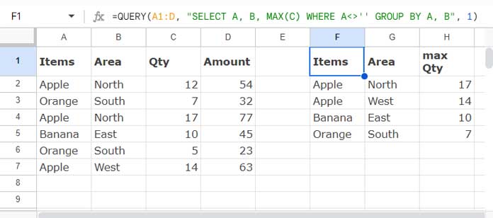
Replace MAX(C) with MIN(C) in the formula if you want to eliminate duplicates based on the minimum quantity rows.
QUERY is not the only function that can eliminate duplicates this way. You can use a combination of SORT and SORTN as follows:
=LET(data, SORT(A2:C, 1, 1, 3, 0, 2, 1), SORTN(data, 9^9, 2, CHOOSECOLS(data, 1)&CHOOSECOLS(data, 2), 1)) // Max
=LET(data, SORT(A2:C, 1, 1, 3, 1, 2, 1), SORTN(data, 9^9, 2, CHOOSECOLS(data, 1)&CHOOSECOLS(data, 2), 1)) // Min
This might be complicated to understand. Please check my corresponding tutorials in my function guide for more detailed explanations.
Another option is unique items and areas while keeping the minimum and maximum quantities. The following formula will do that:
=QUERY(A1:D, "SELECT A, B, MIN(C), MAX(C) WHERE A<>'' GROUP BY A, B", 1)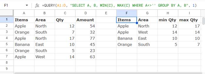
Here, the SORT and SORTN combination won’t meet your requirements.
Wrap-Up
Google Sheets has a built-in tool in the Data menu (Data Clean-up) to remove duplicates from the source data.
If you want the unique rows in a new range, the suggested options are UNIQUE, SORTN, and QUERY.
While QUERY is not specifically designed to remove duplicates, it is an advanced function running a Google Visualization API Query Language query on your data. Its aggregation capabilities allow you to eliminate duplicate rows in ways that UNIQUE or SORTN cannot match.
Resources
- Compare Two Tables and Remove Duplicates in Google Sheets
- How to Remove Duplicates from Comma-Delimited Strings in Google Sheets
- How to Filter Duplicates in Google Sheets and Delete
- Remove Duplicate Values Within Each Row in Google Sheets
- Compare All Columns with Each Other for Duplicates in Google Sheets
- How to Filter Same-Day Duplicates in Google Sheets
It would be great if you actually had the query formula in the post…
Hey, from Br,
thanks for the article.
Did you try in a big sheet, like 10 thousand rows?
I did the same thing using INDEX and FREQUENCY, but it’s very low to calculate entire sheet in each access.
regards
Hi Xico,
Honestly I didn’t test with such a large number of rows!
In between I’ve published a new post on the same subject.
Remove Duplicates in Google Sheets [The Complete Guide and Sample Sheet]
Thanks