")
")


")


")

")
")
 in Excel & Google Sheets")


Did you know that Google Sheets can filter only uppercase, lowercase, or proper case text strings using formulas?
Yes! This tutorial is all about how to filter text based on letter case—a powerful yet lesser-known feature in Google Sheets.
Let’s explore how to extract uppercase, lowercase, and proper case text from a list or table using formulas with the FILTER, EXACT, and REGEXMATCH functions.
Why Filter by Letter Case in Google Sheets?
Filtering by case can help you:
- Identify improperly formatted names or entries.
- Separate ALL CAPS titles from lowercase notes.
- Clean or validate imported data.
And yes, it’s all possible without any Apps Script or add-ons—just formulas.
Case-Sensitive Filtering in Google Sheets – The Basics
To build formulas that distinguish between uppercase and lowercase letters, we’ll use one of these two functions:
EXACT(text1, text2)REGEXMATCH(text, regular_expression)
Both are case-sensitive and return TRUE or FALSE, making them perfect to use as filter conditions. When combined with the UPPER, LOWER, or PROPER functions, we can isolate text strings based on their formatting.
How to Test If Text Is Uppercase, Lowercase, or Proper Case
Test If a Text String Is Uppercase
Let’s say cell B3 contains the text 'APPLE'. The following formulas will return TRUE only if the content is in all capital letters.
Using EXACT:
=EXACT(B3, UPPER(B3))Using REGEXMATCH:
=REGEXMATCH(UPPER(B3), B3)Test If a Text String Is Lowercase
Now, let’s say B3 contains 'apple'. These formulas will check if it’s entirely lowercase.
Using EXACT:
=EXACT(B3, LOWER(B3))Using REGEXMATCH:
=REGEXMATCH(LOWER(B3), B3)Test If a Text String Is Proper Case
Proper case means only the first letter of each word is capitalized (e.g., Prashant Kv).
Using EXACT:
=EXACT(B3, PROPER(B3))Using REGEXMATCH:
=REGEXMATCH(PROPER(B3), B3)How to Filter Uppercase, Lowercase, or Proper Case Text in Google Sheets
Let’s now apply what we’ve learned to filter a list of names based on case.
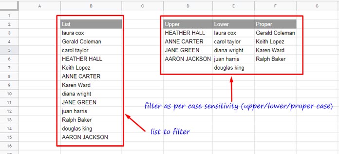
Sample Data: Assume you have a list of names in the range B3:B15. This list may include a mix of uppercase, lowercase, proper case, and even blank cells.
We’ll use the FILTER function with the EXACT function to extract names that match the desired casing.
Note: If the list contains blank cells, these formulas will retain those rows. That’s because EXACT("", UPPER("")) (and similarly with LOWER or PROPER) returns TRUE. You can modify the formulas later to exclude blanks if needed (explained below).
Filter Uppercase Text from a List
=FILTER(B3:B15, EXACT(B3:B15, UPPER(B3:B15)))This formula filters names in B3:B15 that are entirely uppercase, such as HEATHER HALL.
Filter Lowercase Text from a List
=FILTER(B3:B15, EXACT(B3:B15, LOWER(B3:B15)))This returns names like laura cox—entries that are completely in lowercase.
Filter Proper Case Text from a List
=FILTER(B3:B15, EXACT(B3:B15, PROPER(B3:B15)))This filters names like Gerald Coleman, where only the first letter of each word is capitalized.
Optional: Exclude Blank Cells While Filtering
To skip blank rows from appearing in your filtered list, wrap the condition with an ISBLANK check. Here’s how you’d adjust the formula for uppercase text:
=FILTER(B3:B15, EXACT(B3:B15, UPPER(B3:B15)), B3:B15<>"")You can apply the same change to the lowercase and proper case versions by replacing UPPER with LOWER or PROPER.
How to Apply Case-Based Filtering in a Table (Multiple Columns)
All the above examples assume a single-column list. But what if you’re filtering a table like B3:E15?
Just change the first argument of FILTER to the full range, like this:
=FILTER(B3:E15, EXACT(B3:B15, UPPER(B3:B15)))This filters the entire row where column B contains an uppercase string. Replace UPPER with LOWER or PROPER for lowercase or proper case filtering.
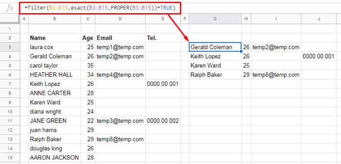
Tip: The condition always checks column B. Adjust as needed if your filter key is in a different column.
Summary: Case-Sensitive Filter Formulas in Google Sheets
| Filter Type | Formula Example |
|---|---|
| Uppercase Only | =FILTER(B3:B15, EXACT(B3:B15, UPPER(B3:B15))) |
| Lowercase Only | =FILTER(B3:B15, EXACT(B3:B15, LOWER(B3:B15))) |
| Proper Case | =FILTER(B3:B15, EXACT(B3:B15, PROPER(B3:B15))) |
These formulas give you full control to filter text based on case sensitivity in Google Sheets—perfect for cleaning data, validating formatting, or segmenting lists.