")


")


")

")
")
 in Excel & Google Sheets")


In Google Sheets, you can filter the top 10 items in a Pivot Table using a custom formula. This formula should be entered in the Custom Formula field under the Pivot Table filter settings.
Before applying the formula, it’s essential to understand how to handle duplicates in the total column, also known as tie-breaking. There are four different tie-breaking options. Review them below and choose the one that fits your needs.
Top N Value Filter in Pivot Table and Tie-Breaking
| Tie-Breaking Mode | Description |
| Mode 0 | Strictly top N |
| Mode 1 | Top N + duplicates of the Nth occurrence (if any) |
| Mode 2 | Unique Top N |
| Mode 3 | Top N + all duplicates |
If you’re unsure which mode to use, refer to the example below, which demonstrates how each mode works when filtering the top 3 items.
Example of Tie-Breaking in a Pivot Table
Let’s consider the top 3 items to illustrate tie-breaking more clearly.
| Product | Qty | Strictly Top 3 (Mode 0) | Top 3 + Duplicates (Mode 1) | Unique Top 3 (Mode 2) | Top 3 + All Duplicates (Mode 3) |
| Product 1 | 50 | ✅ | ✅ | ✅ | ✅ |
| Product 2 | 50 | ✅ | ✅ | ✅ | |
| Product 3 | 40 | ✅ | ✅ | ✅ | ✅ |
| Product 4 | 40 | ✅ | ✅ | ||
| Product 5 | 25 | ✅ | ✅ | ||
| Product 6 | 25 | ✅ | |||
| Product 7 | 20 |
Now that you understand tie-breaking, let’s proceed with an example of filtering the top 10 items in a Google Sheets Pivot Table.
You can access the sample Google Sheet here to follow along. This sheet contains both examples—single-column grouping and multiple-column grouping—along with the Pivot Table setup and formulas used in this tutorial.
For more Pivot Table strategies—including filtering the bottom items, ranking within groups, and custom sorting—see our complete guide: How to Sort and Filter Pivot Tables in Google Sheets.
Example 1: Filter Top 10 Items in a Pivot Table (Single Column Grouping)
Sample Data (Sheet1)
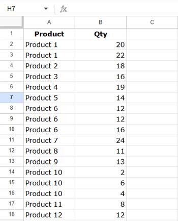
This data will be grouped by Product in the Pivot Table.
Steps to Create a Pivot Table
- Select A1:B.
- Click Insert > Pivot Table.
- In the dialog box, click Create to generate the Pivot Table in a new tab.
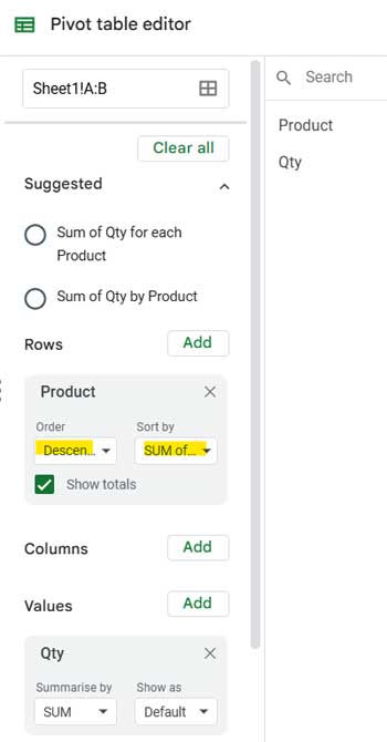
- In the Pivot Table editor:
- Drag Product into the Rows section.
- Drag Qty into the Values section.
- Click the Product field and set the sort order to Sum of Qty (Descending).
Now, let’s apply the filter to display only the top 10 products.
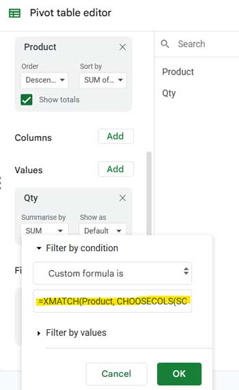
Custom Formula to Filter Top 10 Items in a Pivot Table
=XMATCH(Product, CHOOSECOLS(SORTN(QUERY(QUERY(Sheet1!A1:B, "select Col1, sum(Col2) where Col1 is not null group by Col1 order by sum(Col2) desc"), "offset 1", 0), 10, 0, 2, FALSE), 1))How to Modify the Formula for Your Data
- Replace
Productwith the field label of the grouped column. - Replace
Sheet1!A1:Bwith your actual source data range. - Change the mode (
0,1,2, or3) to suit your tie-breaking preference. The formula currently uses mode 0 (Strictly Top 10).
Applying the Formula
- Open the Pivot Table editor.
- Drag Product to the Filters section.
- Click the dropdown in the Product filter, then select Filter by Condition > Custom Formula is.
- Enter the formula and click OK.
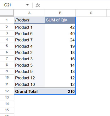
Your Pivot Table will now display only the top 10 items.
Example 2: Filter Top 10 Items in a Pivot Table with Multiple Column Grouping
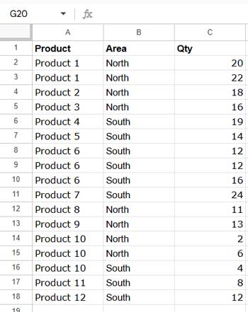
If your dataset contains multiple grouping columns, such as Product and Area, you can still filter the top 10 items.
Sample Data (Sheet2)
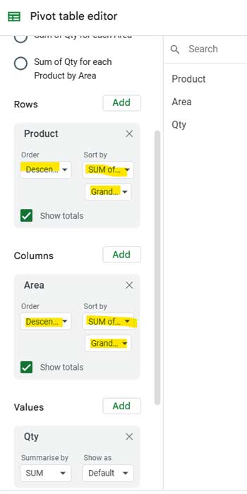
Steps to Create the Pivot Table
- Select A1:C.
- Click Insert > Pivot Table > Create.
- In the Pivot Table editor:
- Drag Product to the Rows section.
- Drag Area to the Columns section.
- Drag Qty to the Values section.
- Set sorting to Sum of Qty > Grand total (Descending) for both Product and Area.
Formula for Filtering Top 10 Items
=XMATCH(Product&Area, LET(sN, SORTN(QUERY(QUERY(Sheet2!A1:C, "select Col1, Col2, sum(Col3) where Col1 is not null group by Col1, Col2 order by sum(Col3) desc"), "offset 1", 0), 10, 0, 3, FALSE), ARRAYFORMULA(HSTACK(CHOOSECOLS(sN, 1)&CHOOSECOLS(sN, 2)))))Modifications
- Replace
Product&Areawith the actual field labels. - Replace
Sheet2!A1:Cwith the correct data range. - Adjust the mode (
0,1,2, or3).
Applying the Filter
- Add Product to the Filters section.
- Use the Custom Formula option and enter the above formula.
- Click OK.
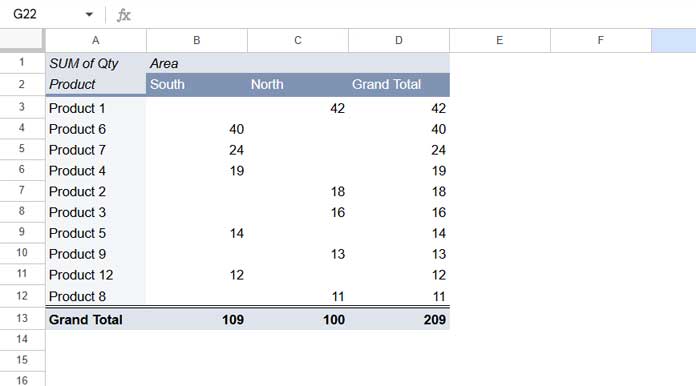
Now, your Pivot Table will filter the top 10 items based on both Product and Area.
FAQs
Will the Pivot Table automatically update when the source data changes?
Yes, the Pivot Table will refresh automatically if you follow the above setup.
Can I use the QUERY function instead of a Pivot Table?
Yes, you can use the QUERY function. However, a Pivot Table offers additional flexibility, such as column and row totals, which would require advanced formulas in QUERY.
How Do I Replace Top 10 with Top 5 or Any Other N?
Simply replace 10 in the formula (before the mode setting) with your desired number N.
Thank You!!!!! This solved my problem.
I’ve been searching everywhere for something like this. 🙂