Filter Rows Containing Multiple Selected Values in Google Sheets

This tutorial explains how to filter rows in a column containing multiple selected drop-down values in Google Sheets.

Assume you have data in two columns: the first column contains customer names, and the second column contains the items each customer bought. You used multiple-selection drop-downs in the second column to select items bought by each customer. This results in multiple items appearing in a row as drop-down chips.

When you want to filter customers who bought a particular item or multiple items, the regular filtering won’t work because of the multiple values in the second column.

Here is how to properly filter rows with multiple selected values in Google Sheets. There are two formulas that handle different scenarios.

Both formulas filter the data based on one or more criteria. However, they differ when multiple selected values exist in the criteria:

The first formula matches either of the selected criteria (OR Logic).
The second formula filters rows that match all selected criteria (AND Logic).

For example:

To filter customers who bought either “Laptop,” “Mouse,” or “Keyboard”, use the first formula.
To filter customers who bought all these items together, use the second formula.
If only one item is selected, both formulas work similarly.

Sample Data

Here is the sample data with customer names in column A and the items bought in column B.

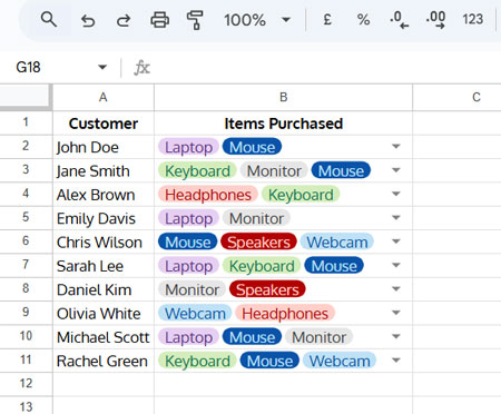
In column B, you can see multiple selected items (drop-down chips). You can create them as follows:

Creating a Multi-Select Drop-Down

First, create a unique list of items in K2:K or any empty column. Then proceed with these steps:

Select the column where you want the drop-down (e.g., B2:B).
Click Insert > Drop-down.
In the sidebar, choose Drop-down (from a range) and select the list of items in K2:K.
Check “Allow multiple selections”.
Click Done.

Specifying the Filter Criteria

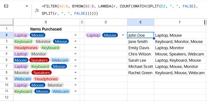
Copy one of the drop-downs, for example, B2, and paste it into D2. Then, select the value(s) you want to filter in D2.

Now, let’s proceed to filter rows with multiple selected values in Google Sheets based on the selected criteria in D2.

Filter Rows with Multiple Selected Values Using OR Logic

To filter rows where at least one of the selected items is present, use this formula:

=FILTER(A2:B, BYROW(B2:B, LAMBDA(r, COUNT(XMATCH(SPLIT(D2, ", ", FALSE), SPLIT(r, ", ", FALSE))))))

How to Test It:

Select the criteria “Laptop” in cell D2. The formula will filter rows where “Laptop” appears in column B (even if other items exist).
If you select “Laptop” and “Mouse” in D2, it will filter rows where either of these items is present.

Example of filtering rows with multiple selected drop-down chips using OR criteria

Formula Breakdown:

The multiple-selected drop-down chips are actually stored as comma-separated values.
To match them, both the criteria (D2) and the data column (B2:B) must be split.
SPLIT(D2, ", ", FALSE) – Splits the criteria into an array.
SPLIT(r, ", ", FALSE) – Splits the current row value in column B into an array.
XMATCH(..., ...) – Matches the split criteria against the split row values and returns an array:
- If an item matches, it returns its relative position.
- If no match is found, it returns #N/A.
COUNT(...) – Counts the number of matches in each row.
The FILTER function returns rows where the count is greater than 0 (indicating at least one match).

This formula correctly filters rows with multiple selected values using OR logic.

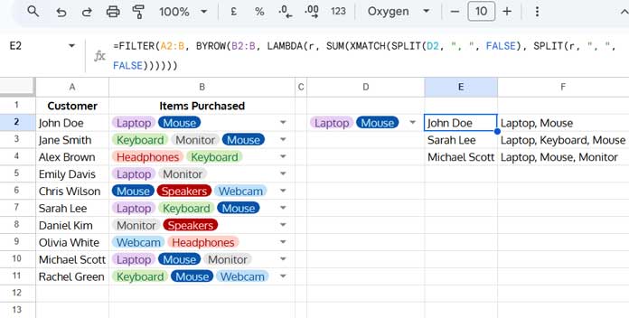
Filter Rows with Multiple Selected Values Using AND Logic

To filter rows where all selected items are present, use this formula:

=FILTER(A2:B, BYROW(B2:B, LAMBDA(r, SUM(XMATCH(SPLIT(D2, ", ", FALSE), SPLIT(r, ", ", FALSE))))))

How It Works:

If you select “Laptop”, the formula filters all rows where Laptop appears in column B.
If you select multiple items, it filters rows where all those items are present.

Example of filtering rows with multiple selected drop-down chips using AND criteria

Logic Behind the Change:

COUNT in an OR-based formula checks for any match.
SUM in this AND-based formula ensures that all selected values are present in the row.

Explanation:

When counting values in a row, if a value matches, it returns 1. COUNT ignores #N/A errors, so it works for an OR condition.
However, when using SUM, the formula returns a sum only if all values match. If any value results in #N/A, the entire sum returns #N/A, filtering out that row.

Example:

Suppose you have a row where column B contains “Laptop, Mouse”.
If the selected criteria are “Laptop, Keyboard”, the formula only returns rows where both exist together.

By refining the AND logic, the formula ensures that only rows containing all selected values are filtered.

Frequently Asked Questions (FAQ)

1. Can I filter based on more than two selected values?

Yes, both formulas dynamically handle multiple selected values.

2. What if my data contains spaces or special characters?

The formulas split values based on ", ", so ensure that your data follows this format.

3. Does this formula work with regular text instead of drop-downs?

Yes, as long as the values are stored as comma-separated text (comma followed by a space).