


")


")

")
")
 in Excel & Google Sheets")


To summarize data in Google Sheets, you can use the QUERY function. However, if you need to extract the top 3, 5, 10, or N values from aggregated QUERY results, a combination of QUERY and SORTN functions is the best approach. The QUERY function aggregates the data, while SORTN extracts the top N values based on different tie-breaking modes.
Using QUERY alone to aggregate data and limit the output to a certain number of rows is not the correct way to extract the top N values from the results.
👉 If you’re unsure when to use LIMIT, SORTN(), or per-group ranking, refer to the complete hub that compares all Top N and row-limiting techniques in Google Sheets QUERY.
When is This Useful?
This method is commonly used in fields such as sales analysis, financial reporting, and performance tracking to extract key insights from aggregated data. Examples include:
- Identifying top-selling products or highest-revenue customers
- Ranking best-performing employees or teams
- Analyzing top expenses or most viewed web pages
By applying this technique in Google Sheets, you can quickly focus on the most important data points for decision-making.
Generic Formula
=SORTN(QUERY(QUERY(data, "select Col1, sum(Col2) where Col1 is not null group by Col1 order by sum(Col2) desc"), "offset 1", 0), n, tie_breaker, 2, FALSE)Explanation:
- Replace
datawith the range where:- The first column contains item names.
- The second column contains numerical values to be totaled.
- Replace
nwith the number of top values to extract. - Replace
tie_breakerwith a value from 0 to 3, depending on how ties should be handled.
The following table explains how the tie_breaker parameter affects the selection of the top N values. Here, N is 5:
| Values | Tie Breaker 0 Stops strictly at N | Tie Breaker 1 Extends to all matching the Nth | Tie Breaker 2 Shows N unique, no duplicates | Tie Breaker 3 Shows N unique, then all duplicates of those |
| 40 | ✅ | ✅ | ✅ | ✅ |
| 40 | ✅ | ✅ | ☑️ | |
| 24 | ✅ | ✅ | ✅ | ✅ |
| 19 | ✅ | ✅ | ✅ | ✅ |
| 18 | ✅ | ✅ | ✅ | ✅ |
| 18 | ☑️ | ☑️ | ||
| 14 | ✅ | ✅ |
Example: Extracting Top N Values from Aggregated Query Results
In the example below, column A contains product names, and column B contains their corresponding quantities.
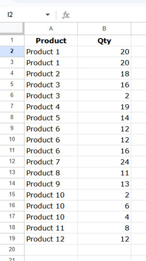
Since some products appear multiple times, we must aggregate the data first before extracting the top N values.
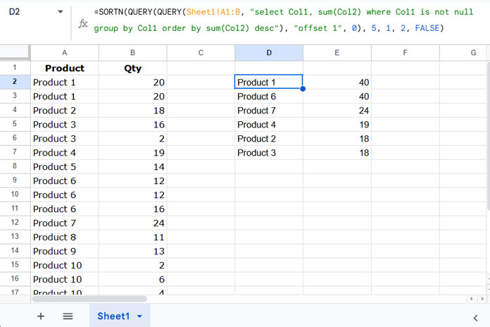
We will filter the top 5 values from the aggregated query results, using tie mode 1 (include ties at Nth value). This approach aligns with how Excel’s Pivot Table handles ties.
Formula:
=SORTN(QUERY(QUERY(Sheet1!A1:B, "select Col1, sum(Col2) where Col1 is not null group by Col1 order by sum(Col2) desc"), "offset 1", 0), 5, 1, 2, FALSE)Result:
Key Takeaways:
- This method ensures that all items meeting the Nth value are included in the output.
- If the Nth value is shared by multiple items (a tie), all such items will be displayed.
- This maintains data integrity and ensures fair representation.
Adjusting Tie-Breaking Modes:
You can modify the tie-breaking mode by changing the 1 in the formula to 0, 2, or 3 as per your needs.
Formula Breakdown:
The formula has three main components and here they are:
1. Aggregation using QUERY:
=QUERY(Sheet1!A1:B, "select Col1, sum(Col2) where Col1 is not null group by Col1 order by sum(Col2) desc")- Groups data by product name (Column 1).
- Sums quantities (Column 2).
- Sorts results in descending order.
2. Removing the header row:
=QUERY(..., "offset 1", 0)- Works like the DROP function in Excel.
3. Extracting the top N values using SORTN:
=SORTN(..., 5, 1, 2, FALSE)- Extracts the top 5 values.
- Uses tie-breaking mode 1 (includes ties at the Nth row).