It’s not tough to construct a regular expression (RE2) to extract negative numbers from different text strings in Google Sheets.

Out of the three related functions, we can use either of the text functions REGEXECTRACT or REGEXREPLACE. No scope for the third one, i.e., REGEXMATCH here.

I think you may have the following queries in your mind to ask. Let me clarify that first.

1. Can we use the extracted negative or positive numbers in other calculations?

We can. For that, we may require to use the VALUE functions to convert the extracted negative numbers in text format to number format.

2. What about multiple (positive or negative) numbers in a text string?

We can extract all of them into multiple columns in the corresponding row.

3. Do you provide an array formula to get negative or positive numbers from a string?

Yep! We can code an array formula using the ArrayFormula function and open/close range within REGEXREPLACE.

Extract All Numbers Irrespective of Their Sign from Text Strings

I have various sample text strings in the range A2:A16. See how to use a non-array formula first to reach our goal.

First of all, select A2:A16 and go to Format> Number > Plain text.

In cell B2, insert the following combo formula and drag it down as far as you want to extract all positive or negative numbers.

=value(ifna(REGEXEXTRACT(A2,"\-?\d*\.?\d+"),))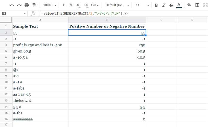

Since our values are in A2:A16, I have dragged this formula until B16.

There are three functions in use in the above formula, and their purposes are as follows.

1. REGEXEXTRACT – Extract numbers irrespective of their sign from the provided text.
2. IFNA – Return blank if the above formula returns #N/A!
3. VALUE – It converts the text formatted numbers (result) into numbers.

Formula Explanation (REGEXEXTRACT)

Here are the explanations to the Regular Expression in use which is,\-?\d*\.?\d+.

\-? – Matches the hyphen character between zero and one time.

\d* – Matches the digit 0-9 between zero or unlimited times.

In the above two, the question mark and asterisk are the quantifiers. In the following two, they are the question mark and the plus sign.

\.? – Matches the period character between zero and one time.

\d+ – Matches the digit 0-9 between one or unlimited times.

Note:-

We can convert the above formula into an array formula.

We can use the below array formula to extract negative or positive numbers from various text strings in Google Sheets.

You may use the below formulas in an empty column, ideally in B2 after emptying B2:B16 or B2:B.

Closed Rage:-

=ArrayFormula(value(ifna(REGEXEXTRACT(A2:A16,"\-?\d*\.?\d+"),)))

Open Range:-

=ArrayFormula(if(A2:A="",,(value(ifna(REGEXEXTRACT(A2:A,"\-?\d*\.?\d+"),)))))

How to Get Multiple Negative or Positive Numbers from Single Text

In the above examples, some of the values in A2:A16 contain multiple numbers.

For example, see cell A4, which contains the numbers 250 and -500.

The above array/non-array formulas only return 250. How do we get both of them?

Here we will use REGEXREPLACE instead of REGEXEXTRACT.

In cell B2, copy-paste the following combo formula and drag it down as far as you want.

=split(REGEXREPLACE(REGEXREPLACE(A2, "[^(\-?\d*\.?\d+)]", "|"),"(\|){1,}","| "),"|")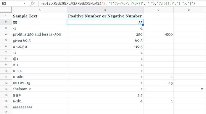

If the formula that extracts negative or positive numbers returns #REF!, hover over the error.

Empty the cell/array the formula is trying to overwrite.

Formula Explanation (REGEXREPLACE)

Earlier, we have used the regular expression \-?\d*\.?\d+ to extract negative or positive numbers in Google Sheets.

Instead, here we have used a negated character class by placing ^ in front of it so that we can replace all the characters except -ve or +ve numbers.

Here is the regular expression for that [^(\-?\d*\.?\d+)].

=REGEXREPLACE(A2, "[^(\-?\d*\.?\d+)]", "|")

In the formula, the pipe is the replacement text/delimiter.

If you use the above formula in cell B4, of course, A2 in it will become A4, the output will be ||||||||||250|||||||||||||-500.

The additional pipe characters will make issues in SPLIT.

So I have used a second REGEXREPLACE with the regular expression (\|){1,} to substitute them.

=REGEXREPLACE(REGEXREPLACE(A4, "[^(\-?\d*\.?\d+)]", "|"),"(\|){1,}","| ")

Output when you use it in cell B4: | 250| -500

Here the replacement text is a pipe and a white space. So in SPLIT also, the delimiter is a pipe with a space.

Related:- How to Remove Extra Delimiter in Google Sheets – Join Columns.

Array Formula:-

=ArrayFormula(IFERROR(split(REGEXREPLACE(REGEXREPLACE(A2:A, "[^(\-?\d*\.?\d+)]", "|"),"(\|){1,}","| "),"|")))

Extracting Negative Numbers Only in Google Sheets

When you follow the above REGEXEXTRACT array or non-array formulas, remove the question mark quantifier immediately after the hyphen to extract only negative numbers in Google Sheets.

Example:

=value(ifna(REGEXEXTRACT(A2,"\-\d*\.?\d+"),))

But it may not work with REGEXREPLACE. There we will use an IF logical test.

=ArrayFormula(
if(
split(REGEXREPLACE(REGEXREPLACE(A2, "[^(\-?\d*\.?\d+)]", "|"),"(\|){1,}","| "),"|")<0,
split(REGEXREPLACE(REGEXREPLACE(A2, "[^(\-?\d*\.?\d+)]", "|"),"(\|){1,}","| "),"|"),
)
)

Note:- The above apply to their corresponding array formulas too.

That’s all. Thanks for the stay. Enjoy!