Extract Every Nth Line from Multi-Line Cells in Google Sheets

It’s not very common to use multiple lines in a single cell—at least in my case—but I do insert multiple lines occasionally. I assume you might do that too. In such cases, it’s helpful to know how to extract every nth line from multi-line cells in Google Sheets.

Table of Contents

What Are Multi-Line Cells in Google Sheets?

If you’re unfamiliar with the term: multi-line cells in Google Sheets refer to cells that contain content across multiple lines—like having multiple rows of text within a single cell.

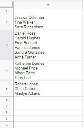
Yes! You can split a single cell into multiple lines and enter different text on each line. Understanding this is essential before we move forward. Here’s a quick example of what multi-line content in a cell might look like:

Cell with multiple lines of text in Google Sheets

How to Create Multiple Lines in a Cell

To insert new lines in a cell, refer to my guide here:
Start New Lines Within a Cell in Google Sheets

In the example (screenshot), we have multiple lines of text in cells C2 to C5. Now, let’s say you want to extract the second line from each of those multi-line cells.

Unlike extracting values from separate rows, it’s not obvious for most users how to pull data from multiple-line cells. Google Sheets doesn’t let you filter text inside a cell like it does with rows. But with the help of formulas, you can extract lines from them.

We’ll use REGEXEXTRACT, which supports RE2 regular expressions, to extract every nth line from multi-line cells in Google Sheets.

Two Approaches: First Line vs Nth Line

The formula to extract the first line from each cell differs from the one used to extract the second, third, fourth, etc. In other words, we need two types of formulas depending on what you’re trying to extract.

Extracting Every Nth Line from Multi-Line Cells in Google Sheets

1. Extracting the First Line

To extract the first line from a multi-line cell, you can use this formula:

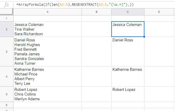
=REGEXEXTRACT(A2, "(\w.*)")

This will extract "Jessica Coleman" from cell A2 if it’s in the first line.

To apply this to a column (e.g., A2:A), use:

=ArrayFormula(IF(LEN(A2:A), REGEXEXTRACT(A2:A, "(\w.*)"), ))

This array formula extracts the first line from each cell in the range A2:A.

Extract every nth line from multi-line cells in Google Sheets

2. Extracting the Second or Nth Line

New lines in a cell are created using the character CHAR(10). Typing:

=CHAR(10)

…into a blank cell will show the line break. While I won’t cover newline creation here (see my earlier linked guide), let’s focus on how to detect and use newline characters in REGEX formulas.

How to Match a New Line Character in REGEX

In Google Sheets, which uses RE2 regular expressions, the newline character is represented as:

\n

To match content after a newline, the regex looks like this:

(\n.*)

This is key to extracting or filtering every nth line from multi-line cells.

Extracting the Nth Line (Other Than First) from a Multi-Line Cell

Let’s say you want to extract the second line from cell A2. Use:

=REGEXEXTRACT(A2, "(\n.*){1}")

This formula extracts the content of the second line, such as "Tina Walker".

To extract the third line, change {1} to {2}:

=REGEXEXTRACT(A2, "(\n.*){2}")

This would extract "Sara Richardson" from the third line.

You can convert this into an array formula to apply it across a column:

=ArrayFormula(IF(LEN(A2:A), REGEXEXTRACT(A2:A, "(\n.*){2}"), ))

This extracts the third line from every cell in the range A2:A.

Handling Errors When the Nth Line Doesn’t Exist

If a cell doesn’t contain an nth line, the formula will return #N/A. To avoid that, wrap the formula with IFNA:

=ArrayFormula(IFNA(IF(LEN(A2:A), REGEXEXTRACT(A2:A, "(\n.*){2}"), )))

This version will return a blank instead of an error if the specified nth line doesn’t exist in a cell.

Conclusion

That’s how you extract every nth line from multi-line cells in Google Sheets using REGEXEXTRACT with newline character handling. Use it to pull out the second, third, or any other specific line from cells that contain multiple lines of text.

9 COMMENTS

Eryk Davidson September 5, 2022 At 12:53 am

Hi,

I’m using the formula:

=RIGHT(REGEXEXTRACT(A1,"(\n.*){14}"), LEN(REGEXEXTRACT(A1,"(\n.*){14}"))-1)

to extract this line from A1: Item Level: 78

Is there any way I can get rid of the “Item Level: ” and just have the number show up?

Thanks,
Eryk

- Prashanth September 5, 2022 At 8:36 am
  
  Hi, Eryk Davidson,
  
  You can try this Regexextract formula.
  
  =regexextract(REGEXEXTRACT(A1,"(\n.*){14}"),"([\d\.]+)")
  
  - Prashanth September 5, 2022 At 9:45 am
    
    Hi, Spencer Barfuss,
    
    Your following formula is correct since you are using the correct Timeofday literal, but you need two fixes.
    
    Your Current Formula:
    
    =query('Form Responses 1'!A2:F,"select * where F < timeofday '"&text(G2,"HH:MM:SS")&"' ORDER BY F",0)
    
    1. Your criteria in cell G2 is a timestamp. It should be a time.
    2. Your source data column F extracts time from column A in that sheet but does not return proper time values.
    
    I have fixed point # 1 above in my sample sheet, i.e., "Copy of Early", in your file.
    
    Regarding point # 2, I have used a virtual column F with proper time values.
    
    Here you go!
    
    =ArrayFormula(query({'Form Responses 1'!A2:E,mod('Form Responses 1'!A2:A,1)}, "select Col1 where Col6 < timeofday '"&text(G2,"HH:MM:SS")&"'",0))
    
J Mann April 10, 2022 At 7:18 am

Thanks – this is great, except that it returns a line of text that begins with a newline.

I stripped the newline by using;

=RIGHT(REGEXEXTRACT(A2,"(\n.*){2}"), LEN(REGEXEXTRACT(A2,"(\n.*){2}"))-1)

Is there a cleaner way to do that?

- Prashanth April 10, 2022 At 12:05 pm
  
  Hi, J Mann,
  
  Simply wrap with TRIM.
  
  =trim(REGEXEXTRACT(A2,"(\n.*){2}"))
  
Gumanjee October 27, 2021 At 2:22 am

Each cell can have a different number of lines. but we know:

1st line is always the NAME.
The penultimate line is always the POSTCODE and CITY.
The last line is always the COUNTRY.

Of course, I can figure out how many lines are there in each cell by counting the next line character.

=LEN(A2)-LEN(SUBSTITUTE(A2,CHAR(10),""))

If the formula returns 4, then there are five lines.

I mean, sure, I can get country for this cell with

=REGEXEXTRACT(A2,"(\n.*){4}")

But the {4} above is manual input, which defeats the purpose.

Ideas?

- Prashanth October 27, 2021 At 10:13 am
  
  Hi, Gumanjee,
  
  You can replace –
  
  =REGEXEXTRACT(A2,"(\n.*){4}")
  
  – with
  
  =REGEXEXTRACT(A2,"(\n.*)"&"{"&LEN(A2)-LEN(SUBSTITUTE(A2,CHAR(10),""))&"}")
  
  I hope the above makes sense.
  
yehonatan Elazar April 5, 2021 At 7:58 pm

Is there a way to choose the LAST line, regardless of how many lines are in the cell?

- Prashanth April 6, 2021 At 8:57 am
  
  Hi, yehonatan Elazar,
  
  You can try this.
  
  =index(split(A2,char(10)),0,COUNTA(split(A2,char(10))))
  
  The formula extracts the last line as follows.
  
  1. Splits values into individual columns based on the new line character.
  split(A2,char(10))
  2. Counts the split values (words).
  COUNTA(split(A2,char(10)))
  3. Using Index, offset the words based on count.