Elapsed Days and Time Between Two Dates in Google Sheets

When you have a start date and time along with an end date and time, you may need to calculate the number of elapsed days and time between the two timestamps.

This is useful for tracking durations, similar to a countdown timer, except instead of using the current time as a reference, you are working with predefined timestamps.

In this tutorial, you’ll learn how to calculate elapsed days, hours, minutes, and seconds between two timestamps in Google Sheets using built-in functions.

Generic Formula to Calculate Elapsed Days and Time

=INT(end-start)&"d "&TEXT(end-start-INT(end-start), "HH:MM:SS")

start – The start date and time.
end – The end date and time.

Example of Calculating Elapsed Days and Time in Google Sheets

To determine the elapsed time between two timestamps, we can use the INT function and TEXT function.

Example Scenario

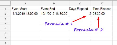
Start Time (A2): 08/01/2019 13:00:00
End Time (B2): 10/01/2019 16:30:00

The elapsed time between these two timestamps is 2 days, 3 hours, and 30 minutes, formatted as:

2d 03:30:00

You can use the following formula in C2 to calculate it:

=INT(B2-A2)&"d "&TEXT(B2-A2-INT(B2-A2), "HH:MM:SS")

Let’s go through the steps to compute this.

Step 1: Calculate Elapsed Days

To get the number of full days elapsed, use this formula in C2:

=INT(B2-A2)

This extracts the integer part of the difference, which represents the number of whole days.

Step 2: Calculate Elapsed Time (Hours, Minutes, Seconds)

To calculate the remaining time beyond whole days, use this formula in D2:

=TEXT(B2-A2-INT(B2-A2),"HH:MM:SS")

This extracts only the time portion of the elapsed duration.

Calculate elapsed time using the INT function in Google Sheets

Step 3: Combine Days and Time

To format the elapsed duration as Xd HH:MM:SS, combine the results of the above formulas:

=C2&"d "&D2

Or, use a single formula for a more compact approach:

=INT(B2-A2)&"d "&TEXT(B2-A2-INT(B2-A2), "HH:MM:SS")

This formula dynamically calculates both days and time in one step.

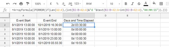
Step 4: Apply an Array Formula for Multiple Rows

If you have multiple rows of start and end times, an ArrayFormula applies the calculation across the entire column:

=ArrayFormula(IF(LEN(A2:A), INT(B2:B-A2:A)& "d "&TEXT(B2:B-A2:A-INT(B2:B-A2:A), "HH:MM:SS"), ""))

This formula ensures that the calculation only applies to non-blank rows, improving efficiency.

Final Output

For multiple timestamps, the output will look like this:

Array formula to calculate elapsed days and time between two dates in Google Sheets