


")


")

")
")
 in Excel & Google Sheets")


Want to cycle highlights in Google Sheets every day? Whether you’re rotating a meal plan, task list, or any repeating schedule, you can use conditional formatting to automatically highlight cells, rows, or columns in a repeating cycle.
For example, imagine you have a meal plan that rotates every 4 days:
- Day 1 ▶ Highlight Menu 1
- Day 2 ▶ Highlight Menu 2
- Day 3 ▶ Highlight Menu 3
- Day 4 ▶ Highlight Menu 4
- Day 5 ▶ Restart from Menu 1
This tutorial will show you how to cycle highlights in Google Sheets across:
- Rows (single cells or full rows)
- Columns (single cells or full columns)
Let’s get started!
Cycle Highlights in Google Sheets Across a Row
[Highlight one cell at a time in a row, moving from left to right daily]
Assume you want to rotate highlights across B3:E6 (4 columns wide).
| Italian | Mexican | Asian | Indian |
Follow these steps:
Step 1: Generate a Date Sequence Across the Row
Enter the following formula in B1 to create a sequence of date values:
=SEQUENCE(1, 4, DATE(2025, 2, 16), 1)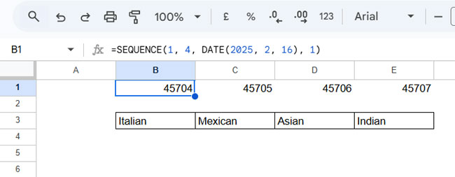
Replace DATE(2025, 2, 16) with today’s date, not using the TODAY function, but in the format DATE(year, month, day).
Step 2: Apply Conditional Formatting
- Select the range B3:E3
- Go to Format > Conditional formatting
- Choose “Custom formula is”
- Enter this formula:
=AND(TODAY()=TODAY()-MOD(TODAY()-B$1,4))- Click Done
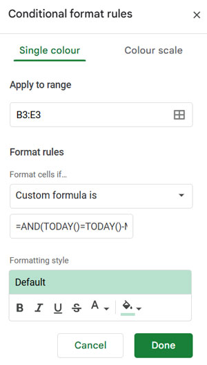
This formula ensures that the highlight moves one cell to the right daily and restarts after 4 days.
Cycle Highlights in Google Sheets for Entire Columns
[Highlight an entire column each day, cycling through a predefined range]
Instead of just highlighting one cell, you may want to highlight full columns daily.
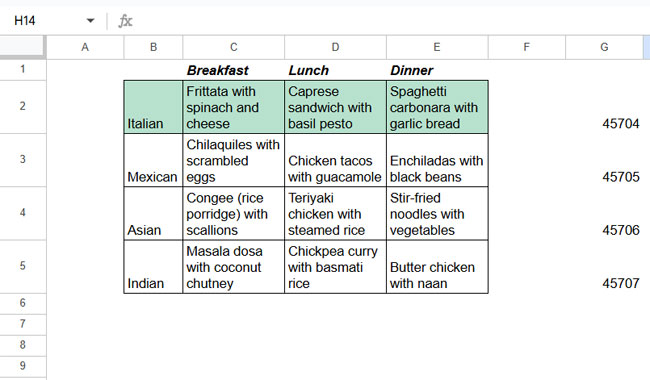
For example, in B3:E6, each column represents a cuisine (B3:E3) with menu items for breakfast, lunch, and dinner listed below (B4:E6), as shown in the image below.
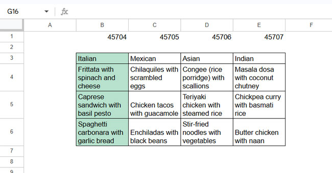
The same formula applies, but the key change is:
Step 1: Apply to the Entire Column Range
In Conditional Formatting, set “Apply to range” as B3:E6 instead of individual cells.
Everything else remains the same, and the highlight will move one column daily and restart after 4 days.
Cycle Highlights in Google Sheets Down a Column
[Highlight one cell at a time in a column, moving downward daily]
Assume you have a list of cuisines in B2:B5:
| Italian |
| Mexican |
| Asian |
| Indian |
To highlight one cuisine per day, follow these steps:
Step 1: Generate a Date Sequence Down the Column
Enter the following formula in G2:
=SEQUENCE(4, 1, DATE(2025, 2, 16), 1)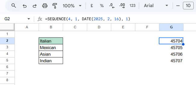
Step 2: Apply Conditional Formatting
- Select B2:B5
- Go to Format > Conditional formatting
- Choose “Custom formula is”
- Enter this formula:
=AND(TODAY()=TODAY()-MOD(TODAY()-$G2,4))- Click Done
Cycle Highlights in Google Sheets for Entire Rows
[Highlight an entire row each day, cycling through a set range]
If you have menu items across the row, you may prefer to highlight entire rows rather than just one cell daily.
For example, in B2:E5, each row contains different meal options.
Step 1: Apply Conditional Formatting to the Entire Row
- Select B2:E5
- Go to Format > Conditional formatting
- Enter the same formula:
=AND(TODAY()=TODAY()-MOD(TODAY()-$G2,4))- Click Done
Now, an entire row will be highlighted each day before cycling back.
FAQs on Cycle Highlights in Google Sheets
1. Can I cycle highlights in Google Sheets without conditional formatting?
No, the best way to cycle highlights automatically is by using conditional formatting with a custom formula.
2. How do I reset the highlight cycle in Google Sheets?
You don’t need to reset it manually—the formulas ensure the cycle continues automatically based on the date.
3. Can I cycle highlights in Google Sheets every X days?
Yes! You can adjust the formula to create an X-day repeating cycle (e.g., a 4-day cycle, 5-day cycle, etc.). This means the highlights will rotate through the specified number of days before starting over, rather than highlighting every Xth day. To customize the cycle length, replace 4 with your desired number in both the SEQUENCE formula and the conditional formatting rule.
Conclusion
In this tutorial, we explored four different ways to cycle highlights in Google Sheets:
- Across rows (one cell or entire rows)
- Across columns (one cell or entire columns)
These formulas help automate rotating highlights for schedules, tasks, meal plans, or any recurring event.
Next Step: Observe the cycle for n+1 days to ensure it loops correctly.